A Practitioner’s Guide to Machine Learning

Deep Learning

We’ve already covered the general principles behind neural networks in a previous chapter. Now we’ll have a look at more complex architectures to work with, for example, image or text data, as well as some advanced training techniques and special-purpose Python libraries for implementing custom neural network architectures.

If you want to learn more about deep learning, there are many great free resources available online, such as the introductory videos from 3blue1brown, which nicely illustrate what neural networks are actually computing and how backpropagation works; the Coursera Deep Learning Specialization (by Andrew Ng), which provides a good general introduction with many practical tips and also covers application areas like computer vision and NLP; or the Deep Learning with PyTorch course (by Yann LeCun), which is a bit more advanced and discusses state-of-the-art architectures.

Advanced NN architectures

Similar to how domain-specific feature engineering can result in vastly improved model performances, it pays off to construct a neural network architecture tailored to the task.

Recurrent Neural Network (RNN)

Recurrent neural networks are great for sequential data such as time series data or text (i.e., a sequence of words).

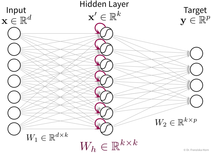
In its simplest form, a RNN is like a FFNN, but with additional recurrent connections \(W_h\) in the hidden layer to create a memory of the past:

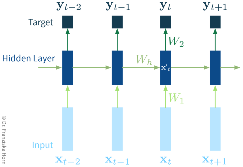
It’s easiest when thinking about the RNN unrolled in time:

At the beginning of a new sequence, the hidden state \(\mathbf{x}'_0\) is initialized with zeros. Then for each new sample \(\mathbf{x}_t\) (with \(t \in \{1, ..., T\}\)) in the sequence, the hidden state is updated based on this new input (after multiplying \(\mathbf{x}_t\) with \(W_1\)), as well as the previous hidden state at \(t-1\) (by multiplying \(\mathbf{x}'_{t-1}\) with \(W_h\)). From this new hidden state \(\mathbf{x}'_t\), the output for this time step can then be predicted (by multiplying \(\mathbf{x}'_t\) with \(W_2\)). While this network only includes a single recurrent layer, a more complex architecture could also contain multiple such layers.

The original RNN layer uses a very simple update rule for the hidden state, but there also exist more advanced types of RNNs, like the Long Short Term Memory (LSTM) network or Gated Recurrent Units (GRU), which define more complex rules for how to combine the new input with the existing hidden state, i.e., they learn in more detail what to remember and which parts to forget, which can be beneficial when the data consists of longer sequences.

The cool thing about RNNs is that they can process input sequences of varying length (where one sequence represents one data point, e.g., a text document), whereas all methods that we’ve discussed so far always expected the feature vectors that represent one data point to have a fixed dimensionality. For RNNs, while the input at a single time step (i.e., \(\mathbf{x}_t\) with \(t \in \{1, ..., T\}\)) is also a feature vector of a fixed dimensionality, the sequences themselves do not need to be of the same length \(T\) (e.g., text documents can consist of different numbers of words). This comes in especially handy for time series analysis, as we’ll see in the next chapter.

Useful in Natural Language Processing (NLP):

RNNs can take word order into account, which is ignored in TF-IDF vectors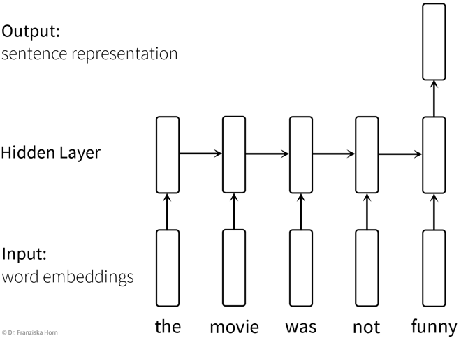: This is an example architecture for a sentence classification task (e.g., sentiment analysis, i.e., deciding whether the text is positive or negative). The individual words in the sentence are represented as so-called word embeddings, which are just d-dimensional vectors that contain some (learned) information about the individual words (e.g., whether the word is more male or female; how these embeddings are created is discussed in the section on self-supervised learning below). The RNN is then fed the sentence word by word and at the end of the sentence, the final hidden state, which contains the accumulated information of the whole sentence, is used to make the prediction. Since the RNN processes the words in the sentence sequentially, the order of the words is taken into account (e.g., whether a “not” occurred before an adjective), and since we use word embeddings as inputs, which capture semantic and syntactic information about the words, similarity between individual words (e.g., synonyms) is captured, thereby creating more meaningful representations of text documents compared to TF-IDF vectors (at the expense of greater computational complexity).

Convolutional Neural Network (CNN)

Manual feature engineering for computer vision tasks is incredibly difficult. While humans recognize a multitude of objects in images without effort, it is hard to describe why we can identify what we see, e.g., which features allow us to distinguish a cat from a small dog. Deep learning had its first breakthrough success in this field, because neural networks, in particular CNNs, manage to learn meaningful feature representations of visual information through a hierarchy of layers.

Convolutional neural networks are very well suited for processing visual information, because they can operate on the 2D images directly and do not need the input to be flattened into a vector. Furthermore, they utilize the fact that images are composed of a lot of local information (e.g., eyes, nose, and mouth are all localized components of a face).

CNNs utilize two important operations, convolutions and pooling layers, to generate meaningful feature representations: A convolution is computed by taking a small filter patch (e.g., a \(5 \times 5\) matrix) and moving it over the image pixel by pixel and row by row, at each position multiplying the filter with the image (see also this animation). This results in a feature map of the same size as the original image, where a high value at some position indicates that the respective feature in the filter (e.g., an edge with a specific orientation) was detected at this position in the original image. Since this is done for multiple filters, the output after a convolutional layer consists of as many new feature maps as the layer had filters. The filter patches (i.e., multiple small matrices) are the learned weights of the CNN, and after training they can look something like the small tiles shown below the network architecture. The pooling layers then perform a subsampling of the individual feature maps by taking the max (or sometimes mean) value of multiple pixels in a small area. This reduces the dimensionality of the hidden layer representation, thereby improving the computational efficiency. Additionally, the pooling introduces some positional invariance, since it is not important anymore where exactly in some area a detected feature was, e.g., a face can be recognized even if the eyes of one person are further apart than usual or they have a longer nose, etc. Usually, the convolutional and pooling layers are interleaved, however, there is no strict rule saying that a pooling layer always has to follow a convolutional layer. With more layers, more and more complex features can be detected as a composition of the features identified in the lower layers (notice how the filters first detect edges, then individual components of a face, then full faces), i.e., by making the network deeper, we can solve more complex tasks. Finally, after multiple convolution and pooling layers, the feature representation is flattened into a vector and fed to a FFNN (i.e., fully connected layers) to perform the classification.

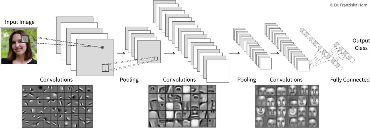
Compared to the dense / fully-connected layers in FFNNs, which consist of one huge matrix mapping from one layer to the next, the filter patches used in convolutional layers are very small, i.e., there are less parameters that need to be learned. Furthermore, the fact that the filters are applied at every position in the image has a regularizing effect, since the filters need to be general enough capture relevant information in multiple areas of the images.

By the way, the edge filters typically learned in the first layer of a CNN nicely match the Gabor filters used in early computer vision feature engineering attempts. Combined with the subsequent pooling operation, they compute something similar as the simple and complex cells in the human primary visual cortex.

General Principles

When trying to solve a problem with a NN, always consider that the network needs to understand the inputs, as well as generate the desired outputs:

As we’ve seen in the CNN used for image classification in the previous section, the representation generated by the CNN is at some point flattened and a FFNN then computes the final prediction for the classification task. Similarly, the final hidden state of a RNN, representing the information contained in a sentences, can be passed to a FFNN to generate a prediction (e.g., for sentiment analysis). However, some problems do not fall into the category of simple supervised learning tasks (i.e., regression or classification), and require a different output. For example, in machine translation, the output should be the sentence translated into the other language, which can be achieved by coupling two RNNs: the first ‘understands’ the sentence in the original language and this representation of the meaning of the sentence is then passed to a second RNN, which generates from it the translated sentence word by word. (If we need to translate texts from and to multiple languages, this can be done very efficiently by using just one input and one output network for each language and have them operate on the same meaning representations, i.e., instead of learning multiple pairs of networks for each language combination individually, we only learn for each language one network to understand this language and one network to generate output sentences in this language.) Another example is the task of image captioning (i.e., generating text describing what can be seen on an image, e.g., to improve the online experience for people with visual impairment), where first the image is ‘understood’ by a CNN and then this representation of the input image is passed to a RNN to generate the matching text.

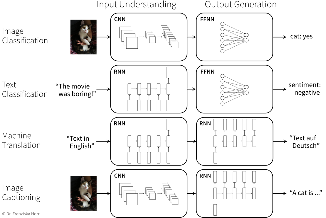
Below are two examples of neural network architectures that deal with somewhat unusual inputs and outputs and incorporate a lot of domain knowledge, which enables them to achieve state-of-the-art performance on the respective tasks:

Predicting the 3D structure of a protein from its amino acid sequence with AlphaFold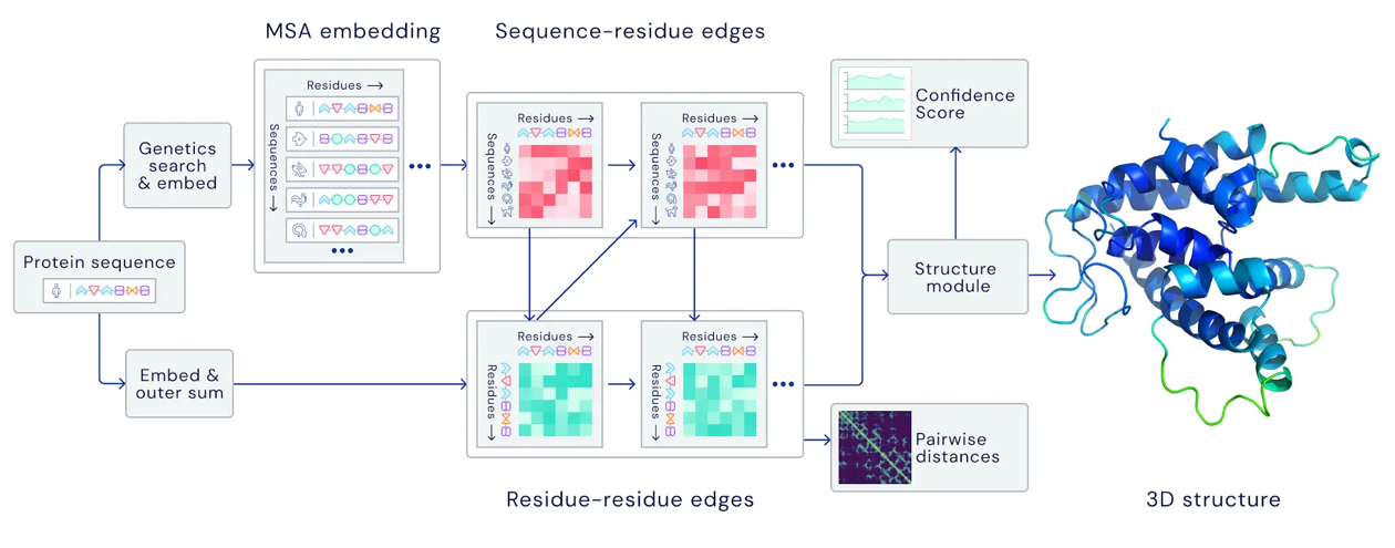: https://deepmind.google/discover/blog/alphafold-a-solution-to-a-50-year-old-grand-challenge-in-biology/ (30.11.2020)
Predicting properties of molecules with SchNet (which is an example of a Graph Neural Network (GNN))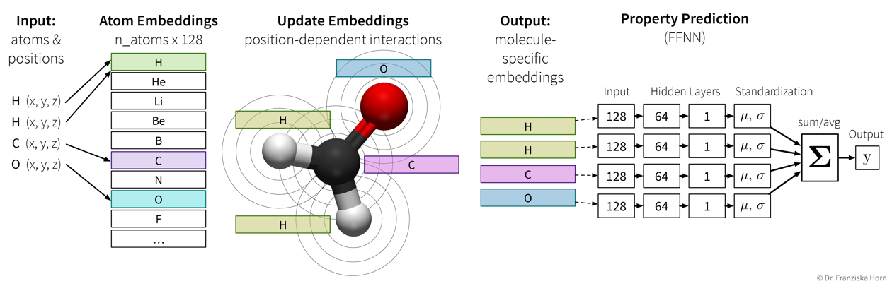: Schütt, Kristof T., et al. “Quantum-chemical insights from deep tensor neural networks.” Nature communications 8.1 (2017): 1-8.

Self-Supervised & Transfer Learning

Self-supervised learning is a very powerful technique with which neural networks can learn meaningful feature representations from unlabeled data. Using this technique is cheap since, like in unsupervised learning, it does not require any labels generated by human annotators. Instead, pseudo-labels are generated from the inputs themselves by masking parts of it. For example, a network can be trained by giving it the first five words of a sentence as input and then asking it to predict what the next word should be. This way, the network learns some general statistics and knowledge about the world, similar to how human brains interpolate from the given information (e.g., with the blind spot test you can nicely observe how your brain predicts missing information from the given context). Self-supervised learning is often used to “pretrain” a neural network before using it on a supervised learning task (see transfer learning below).

NLP Example: Neural Network Language Models (e.g., word2vec → have a look at this blog article for more details) use self-supervised learning to generate word embeddings that capture semantic & syntactic relationships between the words (which is ignored in TF-IDF vectors, where each word dimension has the same distance to all other words):

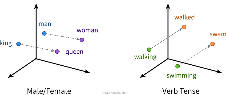
The learned word embeddings can be used to solve analogy questions like those posed in an IQ test, e.g., "man is to king as women is to XXX", where the correct answer is queen. This can be solved with vector arithmetic, i.e., by taking the word embedding for king, subtracting from it the embedding for man, adding the embedding for women and then checking which word embedding is closest to this new vector (which should be the embedding for queen).

⇒ These word embedding vectors can then be used as input to a RNN.

Transfer learning is the idea of using what a network has learned before on a different task (e.g., a self-supervised learning task) as a starting point when tackling a new task. In practice, this means the weights of our network are initialized with (some of) the weights of a network trained on another task, before training our network on the new task. We also say that the network was pretrained on a source task before it is fine-tuned on the target task.

From an old project, we have a network that was trained on a large dataset to recognize dogs in images (= source task). Now we’re working on a new project, where we want to recognize cats in images (= target task). Since the two tasks are very similar (cats and dogs share a lot of the same features) and we only have a small dataset available for the new task, transfer learning could improve the prediction performance on the target task.

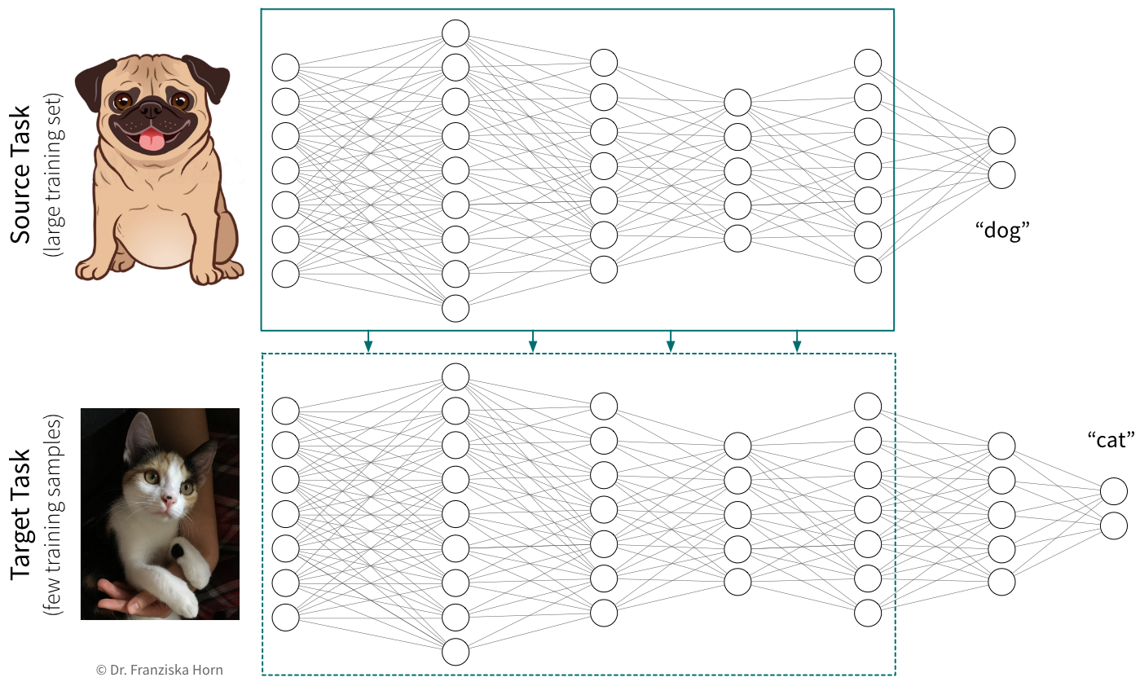
Typically, not all the weights of a target network are initialized with weights from a source network, but only those from the earlier layers, where the source network has learned some general principles that are not task specific (e.g., observe how the first layer of the CNN in the previous section had learned to detect edges, which seems like a relevant skill for pretty much all computer vision tasks). Often, using a pretrained network will give us a more robust solution and boost the prediction performance, especially if we only have a very small dataset for the target task available to train the network. However, since when training a neural network we’re trying to find weights that minimize the loss function by iteratively improving the weights starting with some initialization, if this initialization is unfavorable because it is very far away from a good minimum (i.e., further away than a random initialization), e.g., because we’ve initialized the weights with those from a source network trained on a very different task, then this can hurt the performance, since the network first has to unlearn a lot of things from this unrelated task before it can learn the actual task. Therefore, transfer learning should only be used if the source and target tasks are “related enough”. Pretraining a network on a self-supervised learning task (i.e., a task that is just about understanding the world in general, not solving a different kind of specific task) usually works quite well though.

When using transfer learning, one question is whether to “freeze” the weights that were copied from the source network, i.e., to use the pretrained part of the network as a fixed feature extractor and only train the later layers that generate the final prediction. This is basically the same as first transforming the whole dataset once by pushing it through the first layers of a network trained on a similar task and then using these new feature representations to train a different model. While we often get good results when training a traditional model (e.g., a SVM) on these new feature representations, it is generally not recommended for neural networks. In some cases, we might want to keep the pretrained weights fixed for the first few epochs, but in most cases the performance will be best if all weights are eventually fine-tuned on the target task.

In cases where transfer learning is not beneficial, because the source and target tasks are not similar enough, it can nevertheless be helpful to copy the network architecture in general (i.e., number and shape of the hidden layers). Using an appropriate architecture is often more crucial than initializing the weights themselves.

Neural Networks in Python

There are several libraries available for working efficiently with neural networks (especially since many of the big firms doing machine learning decided to develop their own library): theano was the first major deep learning Python framework, developed by the MILA institute at the university of Montreal (founded by Yoshua Bengio), then came TensorFlow, developed by the Google Brain team, MXNet (pushed by Amazon), and finally PyTorch, developed by the Facebook/Meta AI Research team (lead by Yann LeCun). PyTorch is currently preferred by most ML researchers, while TensorFlow is still found in many (older) applications used in production.

Below you can find some example code for how to construct a neural network using PyTorch or Keras (which is a wrapper for TensorFlow to simplify model creation and training). Further details can be found in the example notebooks on GitHub, which also use the (Fashion) MNIST datasets described below to benchmark different architectures.

[Recommended:] torch library (→ to simplify model training, combine with skorch library!)

import torch
import torch.nn.functional as F

class MyNeuralNet(torch.nn.Module):

    def __init__(self, n_in, n_hl1, n_hl2, n_out=10):
        # neural networks are always a subclass of torch modules, which makes it possible
        # to use backpropagation and gradient descent to learn the weights
        # the call to the super() constructor is vital for this to work!
        super(MyNeuralNet, self).__init__()
        # initialize the layers of the network with random weights
        # a Linear layer is the basic layer in a FFNN with a weight matrix,
        # in this case with shape (n_in, n_hl1), and a bias vector
        self.l1 = torch.nn.Linear(n_in, n_hl1)  # maps from dimensionality n_in to n_hl1
        # we need to make sure that the shape of the weights matches up
        # with that from the previous layer
        self.l2 = torch.nn.Linear(n_hl1, n_hl2)
        self.lout = torch.nn.Linear(n_hl2, n_out)

    def forward(self, x):
        # this defines what the network is actually doing, i.e.,
        # how the layers are connected to each other
        # they are now applied in order to transform the input into the hidden layer representations
        h = F.relu(self.l1(x))       # 784 -> 512 [relu]
        h = F.relu(self.l2(h))       # 512 -> 256 [relu]
        # and finally to predict the probabilities for the different classes
        y = F.softmax(self.lout(h))  # 256 -> 10 [softmax]
        return y

# this initializes a new network
my_nn = MyNeuralNet(784, 512, 256)
# this calls the forward function on a batch of training samples
y_pred = my_nn(X_batch)
# (btw: using an object like a function also works for other classes if you implement a __call__ method)

keras framework (which simplifies the construction and training of TensorFlow networks)

from tensorflow import keras

# construct a feed forward network:
# 784 -> 512 [relu] -> 256 [relu] -> 10 [softmax]
model = keras.Sequential()
# we need to tell the first layer the shape of our input features
model.add(keras.layers.Dense(512, activation='relu', input_shape=(784,)))
# the following layers know their input shape from the previous layer
model.add(keras.layers.Dense(256, activation='relu'))
model.add(keras.layers.Dense(10, activation='softmax'))

# compile & train the model (for a classification task)
model.compile(loss=keras.losses.categorical_crossentropy,
              optimizer=keras.optimizers.Adam(), metrics=['accuracy'])
model.fit(X, y)

# predict() gives probabilities for all classes; with argmax we get the actual labels
y_pred = np.argmax(model.predict(X_test), axis=1)
# evaluate the model (returns loss and whatever was specified for metrics in .compile())
print("The model is this good:", model.evaluate(X_test, y_test)[1])
# but of course we can also use the evaluation functions from sklearn
print("Equivalently:", accuracy_score(y_test, y_pred))

Standard ML Benchmarking Datasets: The MNIST handwritten digits dataset is very old and super easy even for traditional models.
→ \(28 \times 28\) pixel gray-scale images with 10 different classes: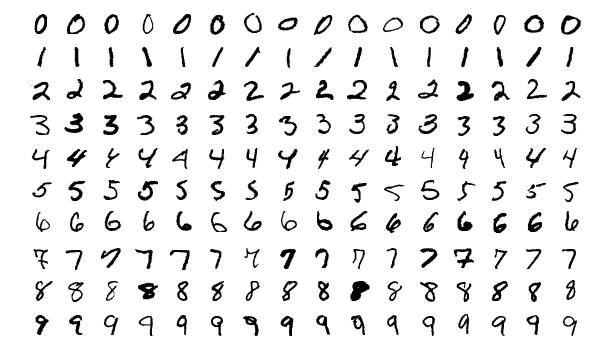

The new MNIST dataset: Fashion
⇒ Same format (i.e., also 10 classes and images of the same shape), but more useful for benchmarks since the task is harder.