Deep Learning

“Deep Learning” describes the subfield of machine learning concerned with neural network models.

Basic Math \[ \small \begin{aligned} \begin{pmatrix} W_{11} & W_{12} & \cdots & W_{1j}\\ W_{21} & W_{22} & \cdots & W_{2j}\\ \vdots & \vdots & \ddots & \vdots\\ W_{i1} & W_{i2} & \cdots & W_{ij}\\ \end{pmatrix} \end{aligned} \]

Dangerous Artificial Intelligence \[ \small \begin{aligned} \begin{pmatrix} W_{11} & W_{12} & \cdots & W_{1j}\\ W_{21} & W_{22} & \cdots & W_{2j}\\ \vdots & \vdots & \ddots & \vdots\\ W_{i1} & W_{i2} & \cdots & W_{ij}\\ \end{pmatrix} \cdot \begin{pmatrix} W_{11} & W_{12} & \cdots & W_{1k}\\ W_{21} & W_{22} & \cdots & W_{2k}\\ \vdots & \vdots & \ddots & \vdots\\ W_{j1} & W_{j2} & \cdots & W_{jk}\\ \end{pmatrix} \cdot \begin{pmatrix} W_{11} & W_{12} & \cdots & W_{1l}\\ W_{21} & W_{22} & \cdots & W_{2l}\\ \vdots & \vdots & \ddots & \vdots\\ W_{k1} & W_{k2} & \cdots & W_{kl}\\ \end{pmatrix} \cdot \begin{pmatrix} W_{11} & W_{12} & \cdots & W_{1m}\\ W_{21} & W_{22} & \cdots & W_{2m}\\ \vdots & \vdots & \ddots & \vdots\\ W_{l1} & W_{l2} & \cdots & W_{lm}\\ \end{pmatrix} \end{aligned} \]

Read on if you’re comfortable with a bit of math. 🤓

Neural Networks

Intuitive Explanation of Neural Networks

[Adapted from: “AI for everyone” by Andrew Ng (coursera.org)]

Let’s say we have an online shop and are trying to predict how much of a product we will sell in the next month. The price we are willing to sell the product for will obviously influence the demand, as people are trying to get a good deal, i.e., the lower the price, the higher the demand; a negative correlation that can be captured by a linear model. However, the demand will never be below zero (i.e., when the price is very high, people wont suddenly return the product), so we need to adapt the model such that the predicted output is never negative. This can be achieved by applying the max function, in this context also called a nonlinear activation function, to the output of the linear model, so that now when the linear model would return a negative value, we instead predict 0.

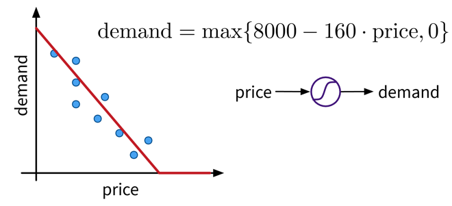
A very simple linear model with one input and one output variable and a nonlinear activation function (the max function).

This functional relationship can be visualized as a circle with one input (price) and one output (demand), where the S-curve in the circle indicates that a nonlinear activation function is applied to the result. We will later see these circles as single units or “neurons” of a neural network.

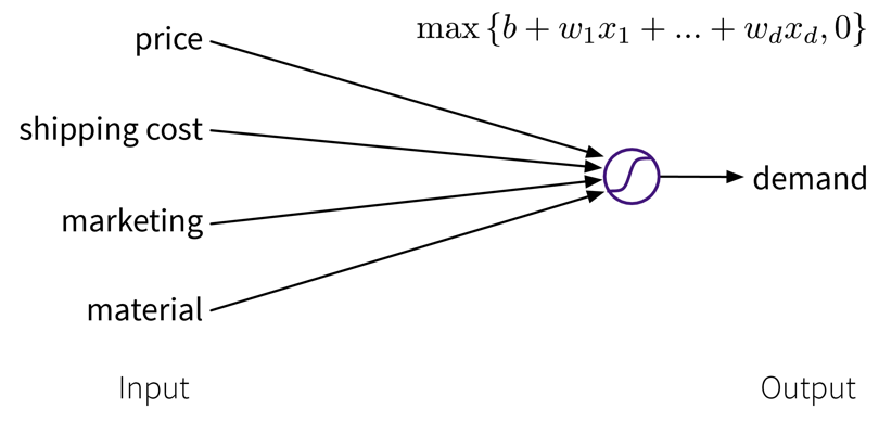
To get better results, we can extend the model and use multiple input features for the prediction:

A linear model with multiple inputs, where the prediction is computed as a weighted sum of the inputs, together with the max function to prevent negative values.

To improve the performance even further, we could now manually construct more informative features from the original inputs by combining them in meaningful ways (→ feature engineering) before computing the output:

Our example is about an online shop, so the customers additionally have to pay shipping fees, which means to reflect the true affordability of the product, we need to combine the product price with the shipping costs. Next, the customers are interested in high quality products. However, not only the actual quality of the raw materials we used to make the product influences how the customers perceive the product, but we can also reinforce the impression that the product is of high quality with a marketing campaign. Furthermore, a high price also suggests that the product is superior. This means by creating these additional features, the price can actually contribute in two ways towards the final prediction: while, on the one hand, a lower price is beneficial for the affordability of the product, a higher price, on the other hand, results in a larger perceived quality.

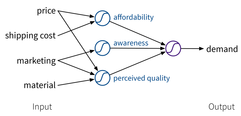
While in this toy example, it was possible to construct such features manually, the nice thing about neural networks is that they do exactly that automatically: By using multiple layers, i.e., stacking multiple linear models (with nonlinear activation functions) on top of each other, it is possible to create more and more complex combinations of the original input features, which can improve the performance of the model. The more layers the network uses, i.e., the “deeper” it is, the more complex the resulting feature representations.

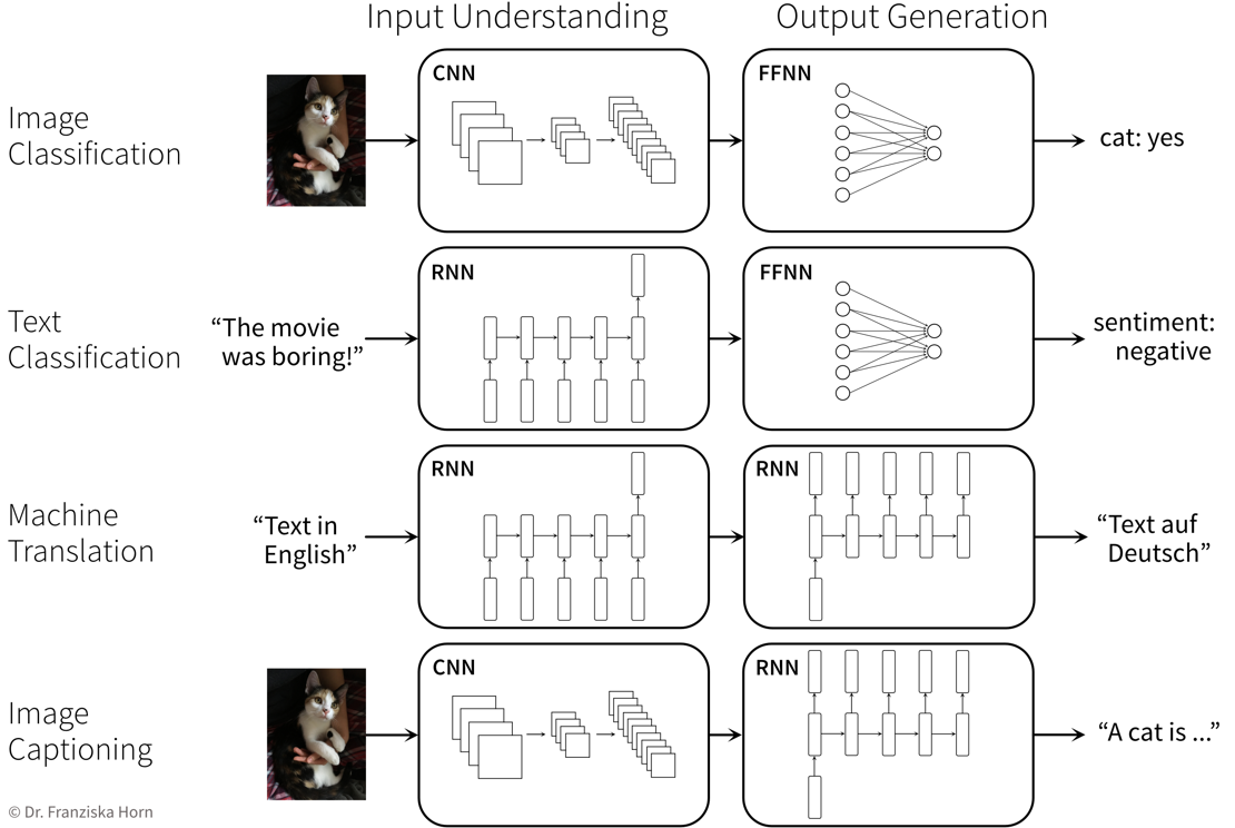
Since different tasks and especially different types of input data benefit from different feature representations, there exist different types of neural network architectures to accommodate this, e.g.

Feed Forward Neural Networks (FFNNs), also called Multi-Layer Perceptrons (MLPs), for ‘normal’ (e.g., structured) data
Convolutional Neural Networks (CNNs) for images
Recurrent Neural Networks (RNNs) for sequential data like text or time series

NN architectures

Similar to how domain-specific feature engineering can result in vastly improved model performances, it pays off to construct a neural network architecture tailored to the task.

Feed Forward Neural Network (FFNN)

This is the original and most straightforward neural network architecture, which we’ve already seen in the initial example, only that in practice such a model usually has a few more layers and units per layer.

Note

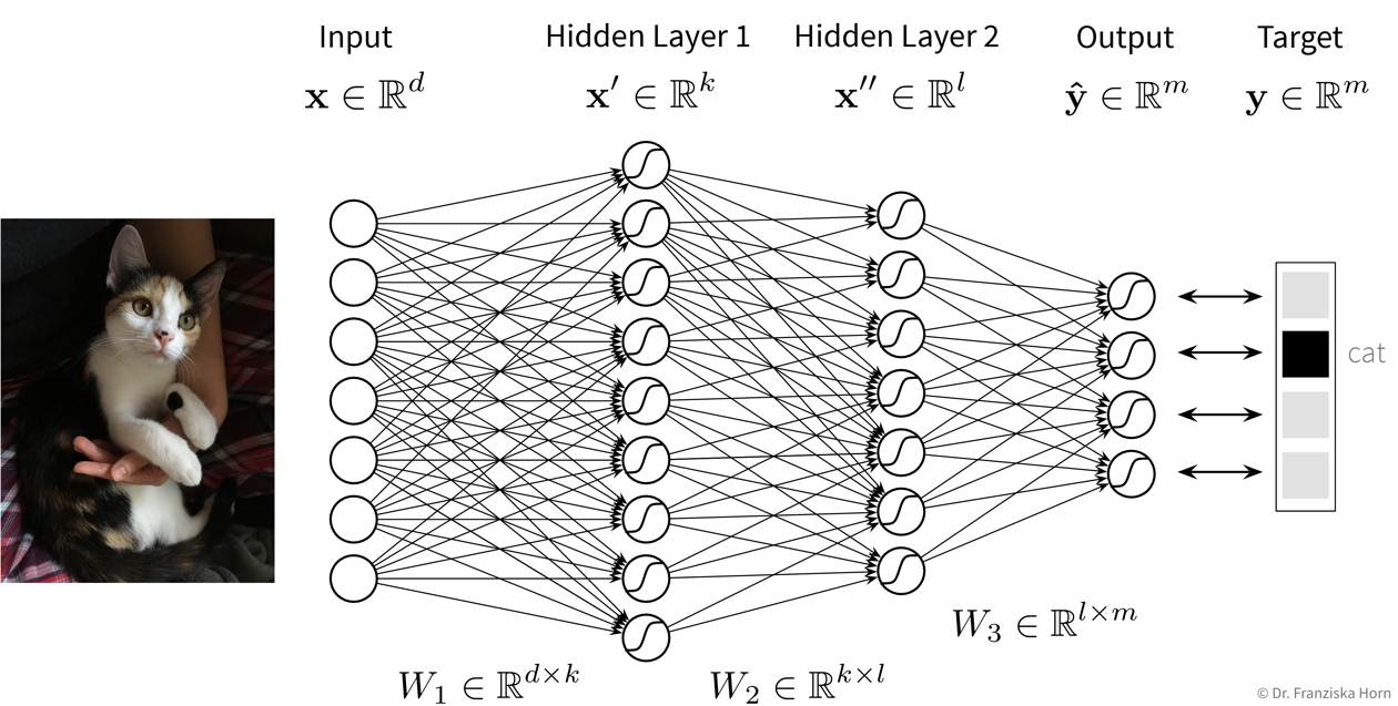
You can play around with a small neural network here to see how it behaves when you, for example, add more units or layers.

Convolutional Neural Network (CNN)

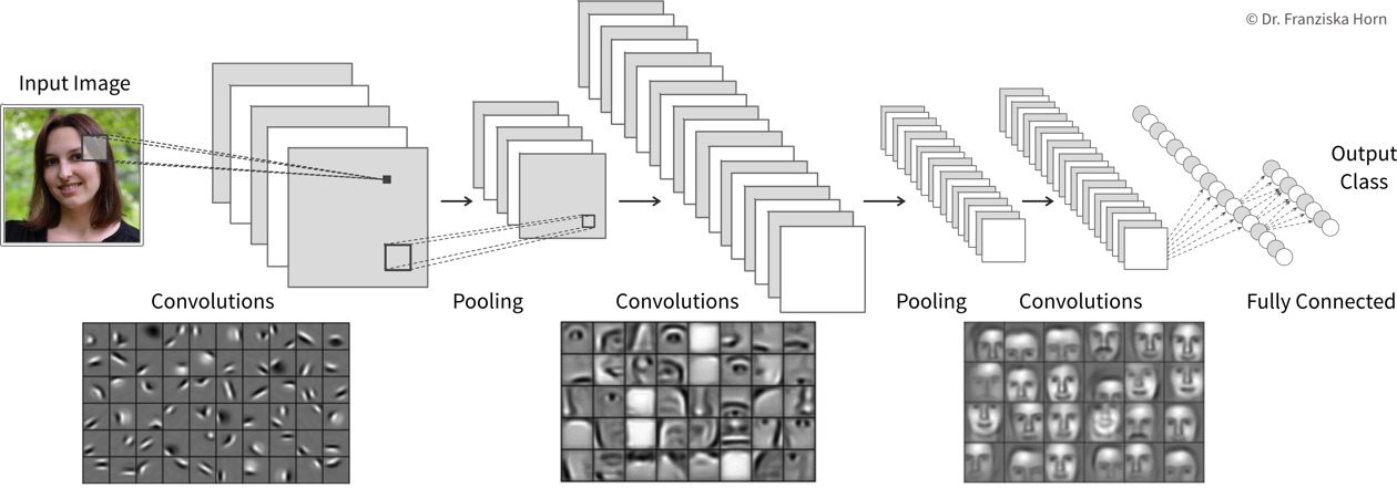
Manual feature engineering for computer vision tasks is incredibly difficult. While humans recognize a multitude of objects in images without effort, it is hard to describe why we can identify what we see, e.g., which features allow us to distinguish a cat from a small dog. Deep learning had its first breakthrough success in this field, because neural networks, in particular CNNs, manage to learn meaningful feature representations of visual information through a hierarchy of layers.

Convolutional neural networks are very well suited for processing visual information, because they can operate on the 2D images directly and utilize the fact that images are composed of a lot of local information (e.g., eyes, nose, and mouth are all localized components of a face).

A convolutional neural network architecture to recognize faces: The learned weights of the network are the small filter patches shown below the network, which, for example, in the first step recognize edges in the image. Towards the end of the network, the feature representation is flattened into a vector and given as input to a FFNN (i.e., fully connected layers) to perform the final classification.

General Principles & Advanced Architectures

When trying to solve a problem with a NN, always consider that the network needs to understand the inputs, as well as generate the desired outputs:

As we’ve seen in the CNN used for face recognition (image classification) above, the representation generated by the CNN is at some point flattened and a FFNN then computes the final prediction for the classification task. Similarly, the final hidden state of a RNN, representing the information contained in a sentences, can be passed to a FFNN to generate a prediction (e.g., for sentiment analysis). However, some problems do not fall into the category of simple supervised learning tasks (i.e., regression or classification), and require a different output. For example, in machine translation, the output should be the sentence translated into the other language, which can be achieved by coupling two RNNs: the first ‘understands’ the sentence in the original language and this representation of the meaning of the sentence is then passed to a second RNN, which generates from it the translated sentence word by word. Another example is the task of image captioning (i.e., generating text describing what can be seen on an image, e.g., to improve the online experience for people with visual impairment), where first the image is ‘understood’ by a CNN and then this representation of the input image is passed to a RNN to generate the matching text.