4 State & Flow: How?
Now that you know what outputs (e.g., result plots) you want to create, are you itching to start programming? Hold on for a moment!
One of the most common missteps I’ve seen junior developers take is jumping straight into coding without first thinking through what they actually want to write. Imagine trying to construct a house by just laying bricks without consulting an architect first—halfway through you’d probably realize the walls don’t align, and you forgot the plumbing for the kitchen. You’d have to tear it down and start over! To avoid this fate for your software, it’s essential to make a plan and sketch out the final design first—to gain clarity on how you could best implement your solution (Figure 4.1).
Your software design doesn’t have to be perfect—we don’t want to overengineer our solution, especially since many details only become clear once we start coding and see how users interact with the software. But the more thought you put into planning, the smoother and faster execution will be.
Unlike a house, where your design will be quite literally set in stone, code should be designed with flexibility in mind. While expanding a house to add extra rooms for a growing family—and then removing them again when downsizing for retirement—would be costly and difficult, this kind of adaptability is exactly what we strive for in software. Our goal is to create code that can evolve with changing requirements.
To make sure your designs will be worthy of implementation, this chapter introduces key paradigms and best practices that will help you create clean, maintainable code that’s easy to extend and reuse in future projects.
Difference Between Commercial Software and Research Code?
Commercial software applications and the scripts used in your research share many of the same core principles—both involve writing code to produce outputs, and both benefit from the same standards of good code quality. That’s the topic of this chapter.
However, full-scale software applications, especially those with graphical interfaces, are naturally more complex than a script that generates static results. The additional components required for production-grade software are covered later in Chapter 6.
Working Code
Before we talk about the best practices for creating good code, let’s first examine what our program is actually supposed to do and which steps we need to execute to produce our desired output—in other words, how to create working code.
Impact Beyond Code
A program would be useless if it did some computation but never revealed the results to anyone. In the end, we always want to produce some kind of effect on the world outside of our code by interacting with users, data stores, or other external systems (Figure 4.2).
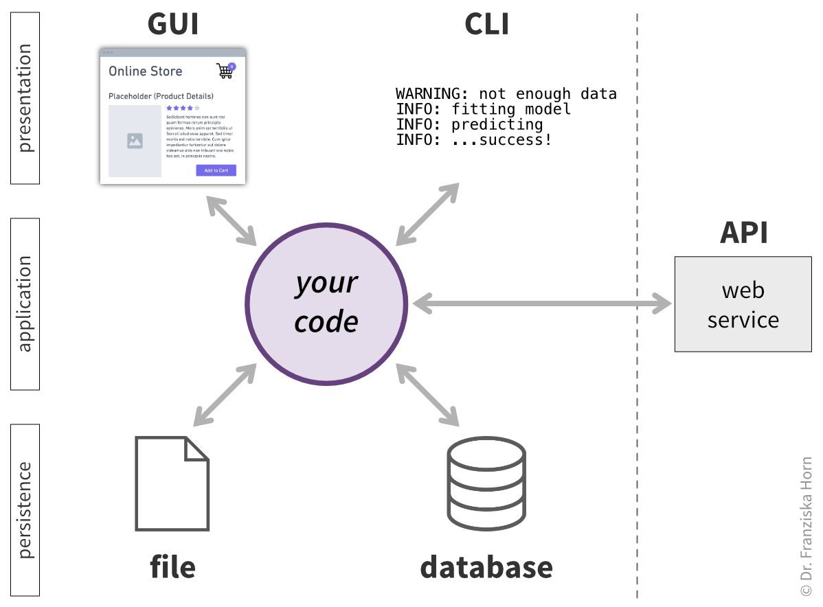
The impact of our code can take many different forms:
- Writing a log message with the result from a calculation to the console.
- Displaying information in a graphical user interface (GUI) and asking the user for input.
- Writing outputs to a file (e.g., an Excel spreadsheet or a PNG image).
- Creating, updating, or deleting records in a database.
- Querying an external web API (e.g., through a POST request).
- Sending an email.
- Transmitting the necessary signals to move the actuators in a robotic arm.
In the previous chapter, we’ve talked at length about what outputs we should show our users to create an optimal user experience. In Chapter 6, we’ll cover how our program can interact with external systems through (web) APIs. So let’s now turn to the topic of data persistence.
Data Persistence
As our code runs, all the data it generates through its calculations and transformations is only present in the computer’s working memory (RAM). Once the program terminates—whether because it is finished with its task or crashes due to an error—these in-memory values are gone. It can therefore be helpful to persist (i.e., save) intermediate results while our code is executed.
Often, intermediate results are also created and consumed by different scripts or processes, for example:
- You run simulations that output data to CSV files. These files are then used by a separate script to generate plots.
- You define model settings in a
config.jsonfile, which your script reads to initialize the model with the correct configuration. - A user fills out a form on a website. Their information is stored in a database so it can later be retrieved and displayed on their profile page.
In these cases especially, it’s important to carefully design the structure of this intermediate data—what fields it includes, what they’re called, and how they’re organized. Because if you later need to change the format, you’ll have to update both the producer and consumer processes, and potentially migrate existing data.
To design an effective structure, start by identifying the fields required by the downstream process. Then consider whether other processes will use this data and if they might need additional fields. You might also want to store the data at a finer level of detail than what’s currently needed. It’s much easier to extract or summarize detailed data later than to reverse-engineer missing details from aggregate values. For example, if you first plan to plot only the final simulation outcome but later want to show values over time, you must have saved the variables at each time step.
If your code is supposed to do more than generate result plots—for example, if you’re running a simulation—you also need to plan your experiment runs.
Think about the data each experiment run will generate and how you’ll process it later. For instance, you might need a separate script that loads data from multiple runs to create additional plots comparing the performance of different models. This is simplified by using a clear naming convention for all output files, such as:
{dataset}_{model}_{model_settings}_{seed}.csvTo determine all possible configuration variants for your experiments, consider:
- The models or algorithms you want to compare (your approach and relevant baselines).
- The hyperparameter settings you want to test for each model.
- The datasets or simulation environments on which you’ll evaluate your models.
- If your setup includes randomness (e.g., model initialization or simulation stochasticity), how many different random seeds you’ll use to estimate variability.
Ideally, your code should allow you to run the same script with different parameter configurations, making it easy to test multiple setups.
If each experiment takes several hours or days, check whether you can run them on a compute cluster and submit each experiment as a separate job to run in parallel.
State & Flow
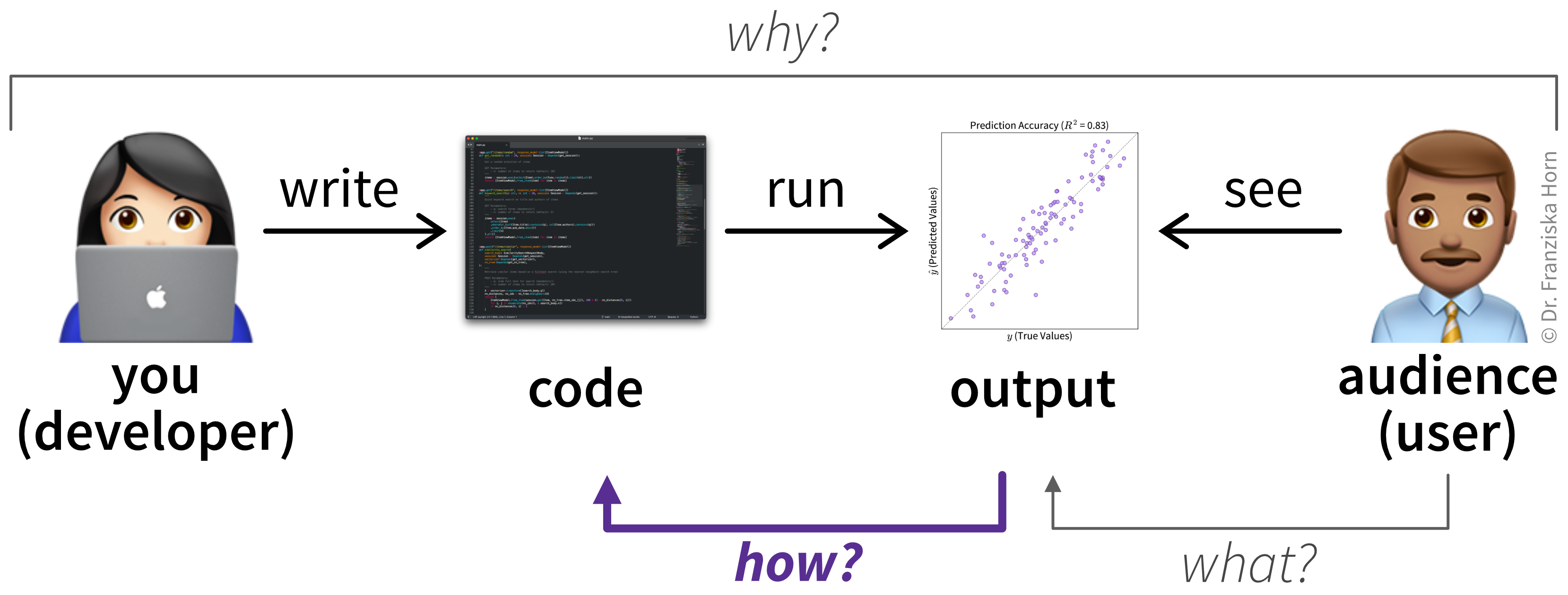
Programming, at its core, is about transforming inputs into outputs [10]. For example, a script could contain the steps needed to turn the data read from a spreadsheet (input) into a result plot shown to the user (output).
To drive this transformation process, the code defines a sequence of operations (e.g., adding or multiplying values), conditional statements (e.g., if/else), and loops (e.g., for and while)—collectively known as an algorithm or control flow.
As these instructions are executed, both the inputs and the intermediate results are stored in variables, which represent the current state of the program.
Data Structures
Variables (like y) store values (like 42). When we initialize a variable, it points to a location in the computer’s memory—a sequence of bits (0s and 1s)—that can be decoded into a specific value. To decode these bits correctly, the system must know the data type of the value being stored. For example, the binary 101010 represents 42 as an integer, but if interpreted as an ASCII character, it yields "*". These data types range in complexity:
- Primitive data types: Simple values like integers or strings (as discussed in Section 3.2.1).
- Composite data types: Structures like lists, sets, and dictionaries that hold multiple values.
- Nonlinear data types: Structures like trees and graphs, used to model complex relationships such as hierarchies or networks.
- User-defined objects: Custom structures defined in classes, tailored for specific use cases.
# primitive data type: float
x = 4.1083

# composite data type: list
my_list = ["hello", 42, x]

# composite data type: dict
my_dict = {
    "key1": "hello",
    "key2": 42,
    "key3": my_list,
}
Depending on the problem you’re solving, choosing the right data structure can make a big difference. For example, structures like trees or graphs can simplify operations such as finding related values or navigating nested relationships. That’s why it’s important to consider not just the sequence of operations in our code, but also how the data is structured.
We can define custom data structures using classes. These are especially useful when multiple values represent a single entity. For instance, instead of managing separate variables like first_name, last_name, and birthdate, we can group them into a single object of a Person class.
While dictionaries could also store related fields, they offer less control: keys and values can be added or removed dynamically and without constraints. In contrast, classes provide structure and validation, such as enforcing required attributes during object creation or controlling how attributes are accessed or updated via class methods.
from datetime import date

class Person:
    def __init__(self, first_name: str, last_name: str, birthdate: date):
        self.first_name = first_name
        self.last_name = last_name
        if birthdate > date.today():
            raise ValueError("Date of birth cannot be in the future.")
        # this attribute is private (by prefixing _)
        # to discourage access outside of the class
        self._bdate = birthdate

    def get_age(self) -> int:
        # code outside the class only gets access to the person's age
        today = date.today()
        age = today.year - self._bdate.year
        if (today.month, today.day) < (self._bdate.month, self._bdate.day):
            age -= 1
        return age

if __name__ == '__main__':
   new_person = Person("Jane", "Doe", date(1988, 5, 20))
This level of control also makes classes a natural choice when an object has distinct states with transitions that must be enforced—in other words, when it acts as a state machine. For example, a machine learning model transitions from untrained to trained when its parameters are fitted on a dataset, and only a trained model should be allowed to make predictions for new data points. A class can enforce this by tracking the current state internally and raising an error on illegal transitions, something a plain dictionary or a collection of loose functions cannot do.
Step by Step: From Output to Input
To determine the sequence of instructions for obtaining our desired outputs, we can work backward to figure out which inputs we need and how these should be transformed (Figure 4.3).
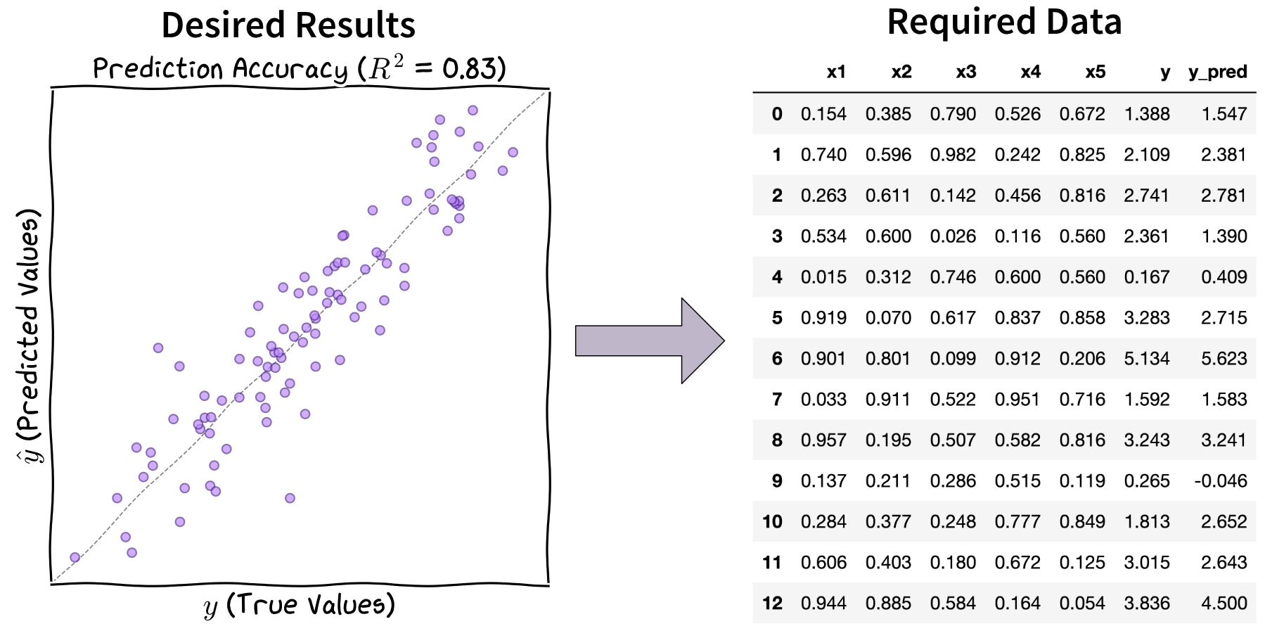
Let’s map out the steps required to create the above scatter plot displaying actual values \(y\) (y), model predictions \(\hat{y}\) (y_pred), and the \(R^2\) value (R2) in the title to indicate the model’s goodness of fit:
To create the plot, we need
R2,y, andy_pred.plot_results(R2, y, y_pred)R2can be computed from the values stored inyandy_pred.R2 = compute_r2(y, y_pred)ycan be loaded from a file containing test data.y = ...y_predmust be estimated using our model, which requires:- The corresponding input values (
x1…x5) from the test data file. - A trained model that can make predictions.
X_test = ... y_pred = model.predict(X_test)- The corresponding input values (
To obtain a trained model, we need to:
- Create an instance of the model with the correct configuration.
- Load the training data.
- Train the model on the training data.
model = MyModel(config)
X_train, y_train = ...
model.fit(X_train, y_train)
The model configuration needs to be provided by the user when running the script.
config = ...
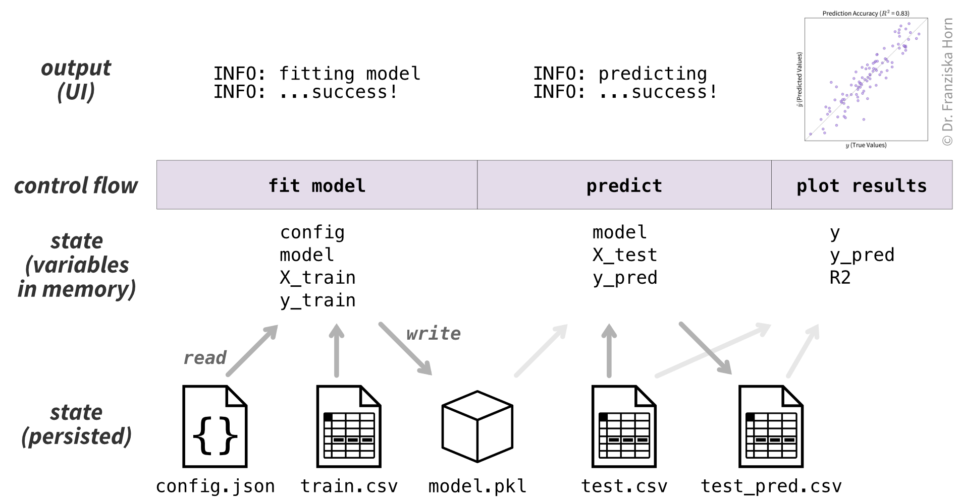
The steps are summarized in Figure 4.4. Of course, in the actual implementation, each step will require further details (e.g., the formula for computing \(R^2\) or how to load the training and test datasets). But since we know that this sequence of transformations will produce the desired output, this already provides us with the rough outline of our code (see Section 4.3 for how these steps could come together in the final script).
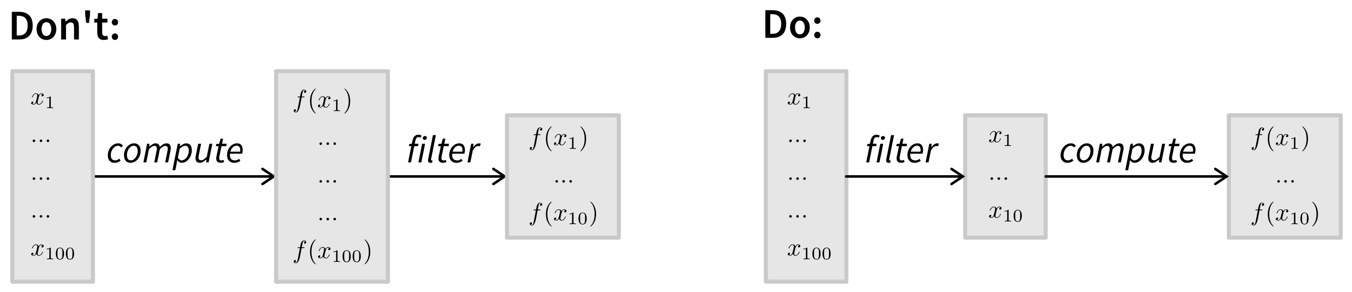
Some steps depend on others (e.g., we must fit our model before making predictions), but others can be performed in any order. Optimizing their sequence can improve performance and efficiency.
For example, if you’re baking bread, you wouldn’t preheat the oven hours before the dough has risen—that would waste energy. Similarly, if you’re processing a large dataset, where you need to perform an expensive computation on each item but only a specific subset of these items is included in the final results, then it may be more efficient to filter the items first so you only compute values for the necessary items:
Designing an Algorithm
Some problems require more creativity to come up with an efficient algorithm that produces the correct output from a given input. Take the traveling salesman problem, where the goal is to find the shortest possible route through a given set of cities. Designing an efficient solution often involves choosing the right data structures (e.g., representing cities as nodes in a graph), using heuristics, and breaking the problem down into simpler subproblems (divide & conquer strategy). If you’re working on a novel problem, studying algorithm design can be invaluable (one of my favorite books on the topic is The Algorithm Design Manual by Steven Skiena [9]).
However, for many common tasks, you can leverage existing algorithms instead of reinventing the wheel. For the rest of this book, we’ll assume you already have a general idea of the steps your code needs to perform and focus on how to implement them effectively.
Coming up with efficient algorithms—even for simple problems—often takes practice. Platforms like LeetCode provide a fun way to build that skill by working through small, focused problems.
While the sequence of steps we derived above enables us to create working code, unfortunately, this is not the same as good code. A script that consists of a long list of instructions can be difficult to read, understand, and maintain. Since you’ll likely be working with the same code for a while—and may even want to reuse parts of it in future projects—it’s worth investing in a better design. Let’s explore how to make that happen.
Good Code
When we talk about “good code” in this book, we focus on three key properties, each building upon and influencing the others:
Easy to understand: To work with code, you need to be able to understand it. When using a common library, it may be enough to know what a function does and how to use it, trusting that it works correctly under the hood. But with your own code, you also need to understand the implementation details. Otherwise, you’ll hesitate to make changes and won’t be able to confidently say that your program behaves as expected. Since code is read far more often than it is written, making it easy to understand ultimately saves time in the long run.
Easy to change: Code is never truly finished. It requires ongoing maintenance—fixing bugs, updating dependencies (e.g., when a library releases a security patch with breaking changes), and adapting to evolving requirements, such as adding new features to stay competitive. Code that is easy to modify makes all of this much smoother.
Easy to build upon and reuse: Ideally, adding new features shouldn’t mean proportional growth in your codebase. Instead, you should be able to reuse existing functionality. Following the DRY (Don’t Repeat Yourself) principle—avoiding redundant logic—also makes code easier to maintain because updates only need to be made in one place.
These qualities (along with others, like being easy to test) can be achieved through encapsulation, i.e., breaking the code into smaller units, and ensuring that these units are decoupled and reusable. This approach has multiple benefits:
- Smaller units fit comfortably into your working memory, making them easier to understand and reason about, which lowers the overall cognitive load of your code.
- Since units are independent, you can change one without unintended side effects elsewhere.
- Well-designed, general-purpose units act as building blocks, allowing you to quickly assemble more complex functionality—like constructing something out of LEGO bricks.
Analogy: The Cupcake Recipe
Before diving into how to write good code, let’s explore some of the basic principles using a more relatable example: a cupcake recipe (Figure 4.6). Because who wants result plots when you could have cupcakes?! 🧁

Like code, a recipe is just text that describes a sequence of steps to achieve a goal. What you ultimately want are delicious cupcakes (your result plots). The recipe (your script) details how to transform raw ingredients (input) into the baked goods (output). But the steps don’t mean anything unless you actually execute them—you have to bake the cupcakes (run python script.py) to get results.
So, how can we write a good recipe?
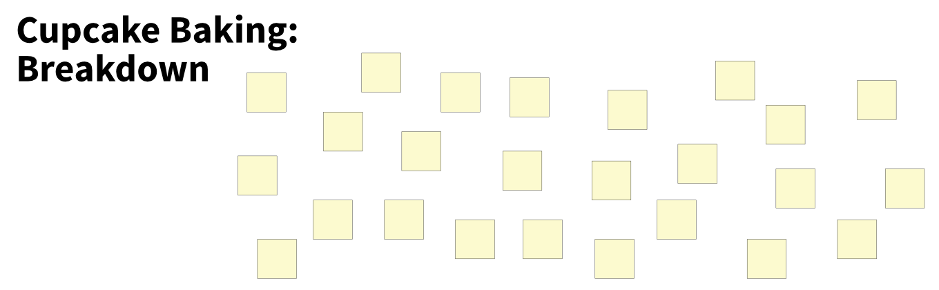
Breaking Down the Steps
To start, we brainstorm all the necessary steps for making cupcakes (Figure 4.7). For this, we can again work backward from the final result (cupcakes) through the intermediate steps (cake batter and frosting) until we reach the raw ingredients.
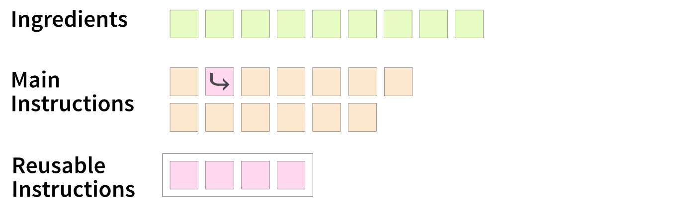
You’ll notice that your list includes both ingredients (in code: variables containing data) and instructions for transforming those ingredients, like melting butter or mixing multiple ingredients (in code: the control flow, i.e., statements, including conditionals (if/else) and loops (for, while), that create intermediate variables). These steps also need to follow a specific order—you wouldn’t frost a cupcake before baking it! Often, steps depend on one another, requiring a structured sequence (Figure 4.8).

Avoiding Repetition: Reusable Steps
If your recipe is part of a cookbook with multiple related recipes, some steps might apply to several of them. Instead of repeating those steps in every recipe, you can group and document them in a separate section (in code: define a function) and reference them when needed (Figure 4.9).
This follows the Don’t Repeat Yourself (DRY) principle [10]. Not only does this reduce redundancy, but it also makes updates easier—if a general step changes (e.g., you refine a technique or fix a typo), you only need to update it in one place (a single source of truth).
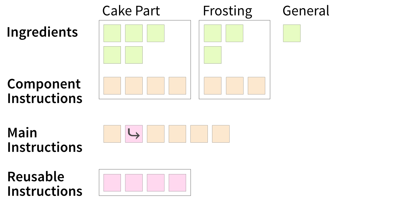
Organizing by Components
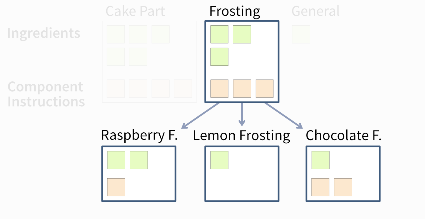
Looking at your recipe, you might notice that some ingredients and instructions naturally group into self-contained components (in code: classes). Structuring the recipe this way makes it clearer and easier to follow (Figure 4.10). Instead of juggling all the steps at once, you can focus on creating one component at a time—first the plain cupcake, then the frosting, then assembling everything.
This modular approach also allows delegation—for example, you could buy pre-made cupcakes and just focus on making the frosting. In programming, this means that the final code doesn’t need to know how each component was made—it only cares that the components exist.
Making Variants with Minimal Effort
Organizing a recipe into components also makes it easier to create variations (Figure 4.11).
Two key concepts make this possible:
- Polymorphism—each variation should behave like the original so it can be used interchangeably (in code: implement the same interface).
- Code reuse—instead of rewriting everything from scratch, extend the original recipe by specifying only the changes (in code: use inheritance or mixins).
For example, a chocolate frosting variant extends the plain frosting recipe by adding cocoa powder. The rest of the instructions remain unchanged.
By applying these strategies, we turn a random assortment of ingredients and instructions into a well-structured, easy-to-follow recipe. This makes the cookbook not only clearer but the recipes also easier to maintain and extend—changes to general instructions only need to be made once, and readers can effortlessly create variations by reusing existing steps.
Now, let’s take the same approach with code.
Encapsulated
Reading through a long script can be overwhelming. To make code easier to understand, we can group related lines into units such as functions and classes—a practice called encapsulation.
Once a block of code exceeds the limits of our working memory, it becomes hard to reason about. Splitting code into functions leverages the fact that our brains handle meaningful chunks far better than long sequences of individual elements. Remembering 177619181945196919892001 is difficult, but grouping the same digits into familiar chunks—1776, 1918, 1945, 1969, 1989, 2001—makes it easy. Functions apply the same principle: they collapse many low-level details into a single, named concept. However, this only works if the chunks are meaningful; splitting code arbitrarily adds indirection and creates confusion.
As a first step, reorder the lines in your code so they follow overarching logical steps, such as data preprocessing or model fitting. For example, if you define a variable at the top of the script, then execute some unrelated computations, and only later use that variable, move the definition down so it’s closer to where it’s actually used. This alone already makes your script easier to follow because the reader doesn’t have to keep unrelated variables in mind while trying to understand what’s happening. You’ll know you’ve succeeded when your code is organized into separate blocks, each representing a distinct process step. You can even add a brief comment above each block describing, at a high level, what the following lines do.
# Before:
df = ...     # data
model = ...  # model

df_processed = ... # do something with df
model_fitted = ... # do something with model

# After:
### Step 1: data preprocessing
df = ...
df_processed = ...

### Step 2: model fitting
model = ...
model_fitted = ...
The next step is to move these blocks into dedicated functions (e.g., preprocessing) or classes (e.g., Model). Done well, this makes your code even more readable: your main script is reduced to a few lines of calls to these units, while the individual functions and classes can be understood in isolation. At that point, you won’t even need the separating comments—your structure will speak for itself.
In the following sections, we’ll explore how to use encapsulation effectively to reduce complexity.
From Complex to Complicated
A well-known software engineering principle is KISS—“Keep It Simple, Stupid!” While this is good advice at the level of individual functions or classes, it’s unrealistic to expect an entire software system to be simple. Most real-world software consists of multiple interacting components, making it inherently complicated rather than simple. The goal is to avoid unnecessary complexity (Figure 4.12).
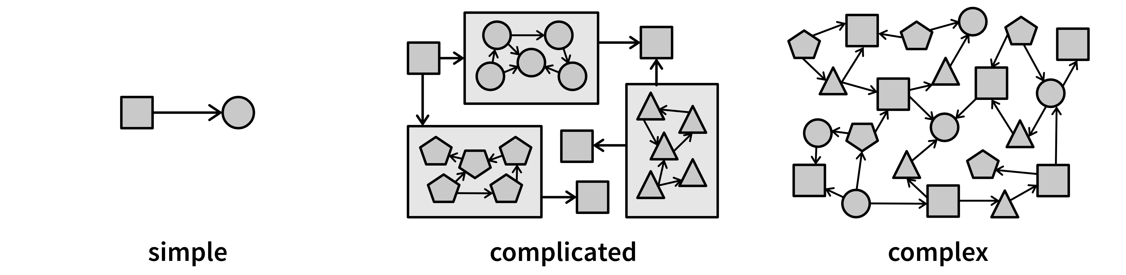
A complex system has many interconnected elements with dependencies that are difficult to trace. Making a small change in one place can unexpectedly break something elsewhere. This makes debugging and maintenance a nightmare.
Instead, we aim for a complicated system—one that may have many components, but is structured into independent, well-organized subsystems [2]. This way, we can understand and modify individual parts without having to fully grasp the entire system.
Decomposing a system this way will always constitute a trade-off, requiring us to balance local vs. global complexity [2]. Consider two extremes:
- A system with two massive 500-line functions has low global complexity (only two things to keep track of) but high local complexity (each function is overwhelming to understand).
- A system with 500 tiny 2-line functions has low local complexity (each function is simple) but high global complexity (understanding how they interact becomes difficult).
What constitutes a “right-sized” unit—small enough to be understandable, yet large enough to avoid excessive fragmentation—will depend on the context and your personal preferences (I usually aim for around 5-15 lines of code, but more complicated algorithms may also justify longer functions). More important than the number of lines, however, is that each unit has a clear, self-contained responsibility.
Following the single responsibility principle, each unit should be cohesive—focused on a single, well-defined task, with all of its internal code serving that purpose.
For example, a cohesive function performs a single task. If a boolean flag in its arguments determines which code path it follows and leads to different return values, it’s better to split it into two separate functions.
Similarly, a cohesive class is designed to represent one specific concept completely—and only that concept. If a class contains many attributes, and one group of methods uses one subset of those attributes while another group relies on a different, non-overlapping subset, this suggests the class no longer adheres to the single responsibility principle and should be broken into smaller, more focused classes.
However, the reverse is also true: units can be too narrowly defined to represent a complete task. For example, if three functions must always run in a specific order to produce a usable result, and none is ever called independently, they should likely be combined into a single function.
Interface vs. Implementation
The key idea of encapsulation is to establish a clear boundary between a unit’s internal logic and the rest of the program. This allows us to hide the complex implementation (the underlying code that users of the unit don’t need to see) behind a simple interface (the part exposed for use). This creates an effective abstraction, reducing cognitive load: users only need to understand how to interact with the unit, not how it works internally.
The interface serves as a contract, promising consistent behavior over time. The implementation, in contrast, is internal and can change freely—so others shouldn’t depend on it.
Let’s look at a simple example to see this in action:
def n_times_x(x, n):
    result = 0
    for i in range(n):
        result += x
    return result

if __name__ == '__main__':
    # call our function with some values
    my_result = n_times_x(3, 5)
    print(my_result)  # should output 15
The interface (also called signature) of the n_times_x function consists of:
- The function name (
n_times_x) - The input arguments (
xandn) - The return value (
result)
Interfaces should be explicit and foolproof, especially since not all users read documentation carefully.
For example, if a function relies on positional arguments, users might accidentally swap values, leading to hard-to-find bugs. Using keyword arguments (i.e., forcing users to specify argument names) makes the interface clearer and reduces errors.
As long as the interface remains unchanged, we can freely modify the implementation. For instance, we can replace the inefficient loop with a proper multiplication:
def n_times_x(x, n):
    return n * x
This change improves efficiency, but since the function still works the same way externally (it’s called with the same arguments and returns the same results), no updates are required in other parts of the code. This is the power of clear boundaries.
However, changing a function’s name, for example, is another story. If we rename n_times_x, every reference to it must also be updated. Modern IDEs can automate this within a project, but if the function is used in external code (e.g., if it is part of an open source library), renaming requires a deprecation process to transition users gradually.
This is why choosing stable, well-thought-out interfaces upfront saves effort in the long run.
In accordance with the principle of information hiding, powerful units have narrow interfaces with deep implementations—they expose only what’s necessary while handling meaningful computations internally [6]. For example:
- A function might take just two inputs (narrow interface) but span ten lines of logic (deep implementation).
- Or a one-liner function might implement a complex formula that users shouldn’t need to understand.
But if your function is called n_times_x, and the implementation is just a one-liner doing exactly that, the abstraction does not help to reduce cognitive load. 😉 As a general rule, a unit’s interface should be significantly easier to understand than its implementation.
Think of calling a function like handing off a task to a colleague: if it takes an hour to explain the relevant context (= many input arguments) so they can complete a task that would have taken you two minutes, the handoff isn’t effective. But if the task requires specialized expertise (= a complex implementation), you’re happy to delegate it to a properly trained colleague and just get the result back.
Class Interfaces
A class groups attributes and methods that belong to a single entity. For well-structured classes, we should carefully control what is public and what is private:
- Public attributes & methods form the external interface—changing them may break code elsewhere.
- Private attributes & methods are meant for internal use and may be modified anytime.
It is often useful to make attributes private and then control how they are accessed or updated through methods. This also implies that any external function that needs to modify an object’s attributes may be better implemented as a method within the corresponding class.
Access levels vary by programming language, for example:
- Java has multiple levels (
public,protected,package,private). - Python relies on convention rather than enforcement. Prefixing names with
_or__signals they are “private”, though they remain accessible.
While Python won’t stop users from accessing private attributes, they do so at their own risk, knowing these details might change without notice.
Decoupled
Two components are connascent [i.e., coupled] if a change in one would require the other to be modified in order to maintain the overall correctness of the system.
– Meilir Page-Jones [7]
We don’t want to just hide arbitrary implementation details behind an interface, but ideally these encapsulated units should also be decoupled. This means they should have as few dependencies as possible on other parts of the code or external resources, especially if these may change frequently. This makes the code easier to understand since each unit can be comprehended in isolation. But even more importantly, it simplifies modifications: when requirements change or new features are needed, we want to minimize the number of places that require updates. In contrast, if code is tightly coupled, a single change in one unit can ripple through multiple parts of the system, increasing the likelihood of errors.
Make Coupling Explicit
To build a larger software system that does something meaningful, we must compose it from multiple components. This inevitably means our units are coupled in some way—one function must call another, so they cannot exist in complete isolation. The goal is to make this coupling explicit so that if one unit changes, it is clear how dependent units need to be updated.
The most explicit form of coupling comes from referencing the public interface of a function or class. Any change in this interface should include a deprecation warning to support a smooth transition for the dependent units. The more explicit the public interface—such as using keyword arguments instead of positional ones—the safer it is to depend on this unit, since compilers and static code analysis tools can detect changes or errors ahead of time, and IDEs can assist with refactoring.
Coupling becomes riskier when your code relies on a unit’s internal implementation details, like private attributes, undocumented quirks, or unintended behaviors (e.g., a function producing odd results when given inputs outside its intended range). Often, multiple parts of a program also share assumptions, such as the meaning of certain values (e.g., the magic number 404 representing the HTTP status code “not found”) or the use of a specific algorithm when encrypting and decrypting data.
The above examples are instances of static coupling, meaning they can be spotted in the source code directly. An even more error-prone form is dynamic coupling, visible only at runtime. For example, a class might require its methods to be called in a particular order to initialize all necessary values for a correct computation.
To minimize coupling risks, identify the assumptions your code makes about how and in which context it will be used. Don’t just document the correct usage and hope it’s followed, but make interactions explicit. This can mean defining formal interfaces, validating inputs, and enforcing usage constraints in code. Otherwise, the system becomes fragile, and even small changes in unrelated areas can cause breakages.
Levels of Abstraction
Ideally, our units should form a hierarchy with different levels of abstraction (Figure 4.13), where lower-level units can be used as building blocks to create more advanced functionality.
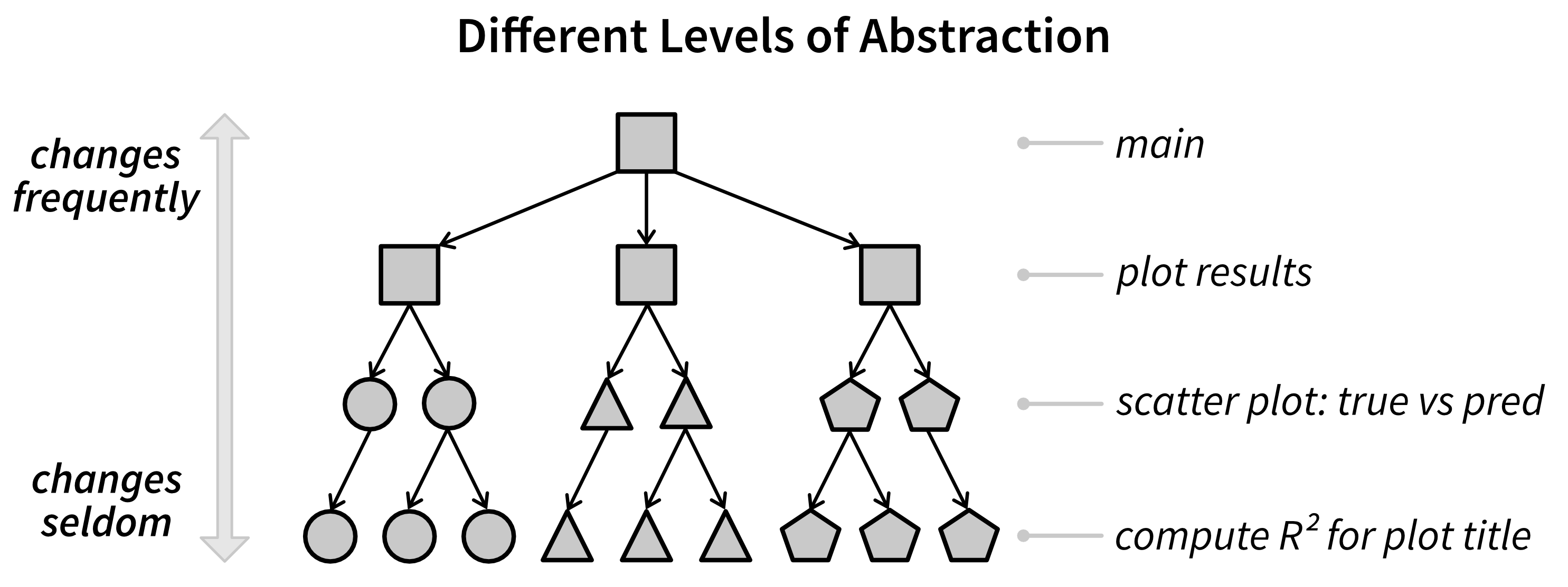
At each level, you only need to understand how to use the functions at lower levels but not their internals. This reduces cognitive load, making it easier to navigate and extend the codebase with confidence.
However, it’s important to note that low-level functions should ideally be kept stable, since everything built on top of them depends on their behavior. If the interface of such a function changes, any code that relies on it will also need to be updated. This applies not only to your own functions but also to external libraries your code depends on.
Standard libraries (i.e., those included with a programming language, not installed separately) are generally safe to build upon, as their functionality tends to be stable. In contrast, relying heavily on experimental or rapidly evolving libraries can lead to constant breakage as new versions introduce changes. To mitigate this, consider implementing an anti-corruption layer—a wrapper that provides a stable interface and handles necessary transformations when interacting with third-party code. This centralizes adaptation and isolates the rest of your code from volatile dependencies.
Maintaining a clear hierarchy of abstraction also helps prevent circular dependencies—situations where two or more modules depend on each other, either directly or indirectly. Such dependencies break modular design: a change in one component can ripple unpredictably through others, making the system harder to reason about, test, and maintain. They also complicate initialization and reduce flexibility, since no component can evolve independently. Establishing clean dependency directions—where higher-level modules depend on lower-level ones, but not vice versa—keeps the architecture stable and comprehensible.
Pure vs. Impure Functions
In addition to dependencies on code defined elsewhere, another form of coupling comes from relying on external resources (like files, databases, or APIs), which may also change frequently. These kinds of external dependencies are eliminated when our units are pure functions [5].
A pure function behaves like a mathematical function \(f: x \to y\), taking inputs \(x\) and returning an output \(y\)—and given the same inputs, the results will be the same every time. Impure functions, on the other hand, have side effects—they interact with the outside world, such as reading from or writing to a file or modifying global state.
def add(a, b):
    # pure: returns a computed result without side effects
    return a + b

def write_file(file_path, result):
    # impure: writes data to a file (side effect)
    with open(file_path, "w") as f:
        f.write(result)
Why favor pure functions? First, they are predictable—calling them with the same inputs always produces the same output, unlike impure functions, which may depend on changing external factors (e.g., the function may run fine the first time but then crash when trying to create a file that already exists or the computed results are suddenly different because in the meantime other code updated values stored in a database). Second, they are easy to test since they don’t rely on external state, as we’ll show below.
That said, impure functions are often necessary—code needs to have an effect on the outside world, otherwise why should we execute it in the first place? The trick is to encapsulate as much essential logic as possible in pure functions at the lower levels of abstraction, while isolating side effects in higher levels:
def pure_function(data):
    # process data (pure logic)
    result = ...
    return result

def impure_function():
    with open("some_input.txt") as f:
        data = f.read()
    result = pure_function(data)
    with open("some_output.txt", "w") as f:
        f.write(result)
This structure ensures the core logic is pure and testable:
# tests.py
def test_pure_function():
    data = "some test data"
    result = pure_function(data)
assert result == "some test result"A related design heuristic is command-query separation: functions that return information (queries) should not change state, and functions that change state (commands) should do minimal computation. Pure functions are natural queries—they observe data and return a result without side effects. Impure functions that write to files, databases, or external services are commands. Keeping these roles strictly separate makes code easier to reason about: you can call a query as often as you like without worrying about side effects, and commands become simpler when they don’t also contain complex logic.
Dependency Injection for Flexibility
To further decouple your code, use dependency injection [8]: instead of hardcoding dependencies (e.g., file operations, database access), pass them as arguments. This allows functions to remain independent of specific implementations.
Without dependency injection:
class DataSource:
    def read(self):
        with open("some_input.txt") as f:
            return f.read()
    def write(self, result):
        with open("some_output.txt", "w") as f:
            f.write(result)

def fun_without_di():
    # create external dependency inside the function
    ds = DataSource()
    data = ds.read()
    result = ...
    ds.write(result)
With dependency injection:
def fun_with_di(ds):
    # dependency is passed as an argument
    data = ds.read()
    result = ...
    ds.write(result)

if __name__ == '__main__':
    ds = DataSource()
    fun_with_di(ds)
Now, fun_with_di only requires an object implementing read and write, but it doesn’t care if it’s a DataSource or something else that implements the same interface. This makes testing much easier:
# tests.py
class MockDataSource:
    def read(self):
        return "Mocked test data"
    def write(self, result):
        self.success = True

def test_fun_with_di():
    mock_ds = MockDataSource()
    fun_with_di(mock_ds)
    assert mock_ds.success
Dependency injection can also be combined with pure functions to make your code testable at different levels of abstraction (Figure 4.14).
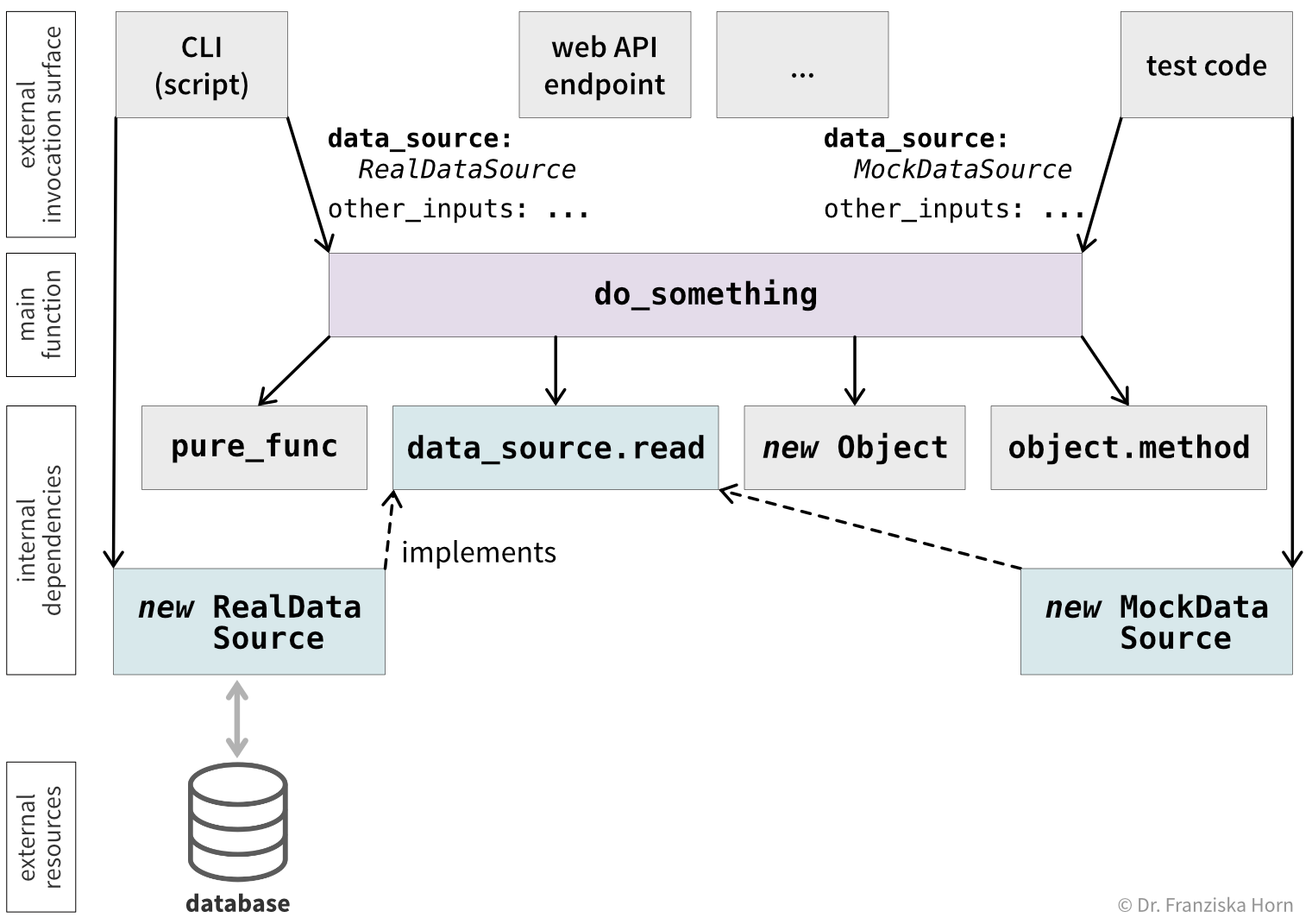
do_something) can be invoked through multiple entry points, such as a CLI script, a web API endpoint, or test code. Each entry point constructs a data_source object—either a RealDataSource with database access or, in tests, a MockDataSource—which is then passed to do_something, where data_source.read is called. But do_something does not directly depend on RealDataSource or MockDataSource.
This approach also makes it straightforward to extend your code by integrating additional data sources through wrappers that share the same interface. For example, if you switch to a different type of database, you only need to implement a new wrapper class and initialize it in the outer calling code; the main function and its dependencies can remain unchanged.
A key point here is to design your code for testability by abstracting access to external resources that should not be touched during tests. While it often makes sense to introduce dedicated wrappers for complex data sources such as databases, simpler cases do not always require this level of abstraction. If your function only reads from a CSV file, it may be sufficient to pass the file path as an argument and use a separate, smaller test file when running tests.
Anti-Pattern: Global Variables
Besides external resources like files and databases, another source of tight coupling and error-prone behavior is relying on global variables. These are defined at the script level (often below import statements) and can be accessed or modified anywhere in the code.
Global variables can introduce temporal coupling, meaning the order of function execution suddenly matters. This can lead to subtle and hard-to-debug issues:
PI = 3.14159

def calc_area_impure(r):
    # since PI is not defined inside the function,
    # the fallback is to use the global variable
    return PI * r**2

def change_pi(new_pi=3):
    # `global` is needed to not create a new local variable
    global PI
    PI = new_pi

if __name__ == '__main__':
    r = 5
    area_org = calc_area_impure(r)
    change_pi()
    area_new = calc_area_impure(r)
    assert area_org == area_new, "Unexpectedly different results!"
The safer approach is to pass values explicitly:
def calc_area_pure(r, pi):
    return pi * r**2
This avoids hidden dependencies and ensures reproducibility.2
To prevent unintended global variables, wrap your script logic inside a function:
def main():
   # main script code incl. variable definitions
   ...

if __name__ == '__main__':
    main()
This ensures that variables defined inside main() don’t leak into the global namespace.
If multiple functions need to update the same set of variables, consider grouping them into a class instead of relying on globals. A class can store shared state in attributes, accessed via self, which is especially important if this shared state should change over time through a defined set of operations (like a state machine), where the class can enforce valid transitions and keep the state consistent.
🚨 Call-By-Value vs. Call-By-Reference
Another common pitfall is accidentally modifying function arguments.
Depending on the programming language you use, input arguments are passed:
- By value: A copy of the data is passed.
- By reference: The function gets access to the original memory location and can modify the data directly.
Python uses call-by-reference for mutable objects (e.g., lists, dictionaries), which can lead to unexpected behavior:
def change_list(a_list):
    a_list[0] = 42  # modifies the original list
    return a_list

if __name__ == '__main__':
    my_list = [1, 2, 3]
    print(my_list)  # [1, 2, 3]
    new_list = change_list(my_list)
    print(new_list) # [42, 2, 3]
    print(my_list)  # [42, 2, 3] 😱
To prevent such side effects, create a copy of the variable before modifying it. This ensures the original remains unchanged:
from copy import deepcopy

def change_list(a_list):
    a_list = deepcopy(a_list)
    a_list[0] = 42
    return a_list

if __name__ == '__main__':
    my_list = [1, 2, 3]
    new_list = change_list(my_list)
    print(my_list)  # [1, 2, 3] 😊
To avoid sneaky bugs, test your code to verify:
- Inputs remain unchanged after execution.
- The function produces the same output when called twice with identical inputs.
Don’t Repeat Yourself (DRY)
A more subtle form of coupling comes from violating the DRY (Don’t Repeat Yourself) principle. For example, critical business logic—such as computing an evaluation metric, applying a discount in an e-commerce system, or validating data, like the rules that define an acceptable password—might be duplicated across several locations. If this logic needs to change (due to an error or evolving business requirements), you’d need to update multiple places, making your code harder to maintain and more prone to bugs. To avoid inconsistencies and duplicated work, make sure that important values and business rules are defined in a central place, the single source of truth.
The most obvious DRY violation occurs when you catch yourself copy-pasting code—this is a clear signal to refactor it into a reusable function. However, DRY isn’t just about code; it applies to anything where a single change in requirements forces multiple updates, including tests, documentation, or data stored across different databases [10]. To maintain your code effectively, aim to make each change in one place only. If that’s not feasible, at least keep related elements close together—for example, documenting interfaces using docstrings in the code rather than in separate files.
Reusable
While we want to keep interfaces narrow and simple, we also want our units to be broadly applicable. This often means replacing hardcoded values with function arguments. Consider these two functions:
def a_plus_1(a):
    return a + 1

def a_plus_b(a, b=1):
    return a + b
The first function is highly specific, while the second is more general and adaptable. By providing sensible default values (b=1), we keep the function easy to use while allowing flexibility for more advanced cases.
Reusable code isn’t typically created on the first try because future needs are unpredictable. Instead of overengineering, focus on writing simple, clear code and adapt it as new opportunities for reuse emerge. This process, called refactoring, is covered in more detail in Section 5.7.
That said, if your function ends up with ten arguments, reconsider whether it really has a single responsibility. If it’s doing too much, breaking it into multiple functions is likely a better approach.
Polymorphism
When working with classes, reuse can be achieved through polymorphism, where multiple classes implement the same interface and can be used interchangeably. We’ve already applied this principle when we used MockDataSource instead of DataSource for testing. This approach can be useful in research code as well, for example, you could define a Model interface with fit and predict methods so multiple models can share the same experiment logic:
class Model:
    def fit(self, x, y):
        raise NotImplementedError
    def predict(self, x):
        raise NotImplementedError

class MyModel(Model):
    def fit(self, x, y):
        ...  # implementation
    def predict(self, x):
        y_pred = ...
        return y_pred

def run_experiment(model: Model):
    # this code works with any model that implements
    # appropriate fit and predict functions
    x_train, y_train = ...
    model.fit(x_train, y_train)
    x_test = ...
    y_test_pred = model.predict(x_test)

if __name__ == '__main__':
    # create a specific model (possibly based on arguments
    # passed by the user when calling the script)
    model = MyModel()
    run_experiment(model)
This way you can reuse your analysis code with all your models, which not only avoids redundancy, but ensures that all models are evaluated consistently.
Mixins
Another approach to reuse is using mixins—small reusable classes that provide additional functionality:
import numpy as np

class ScoredModelMixin:
    def score(self, x, y):
        y_pred = self.predict(x)
        return np.mean((y - y_pred)**2)

class MyModel(Model, ScoredModelMixin):
    ...

if __name__ == '__main__':
    model = MyModel()
    # this uses the function implemented in ScoredModelMixin
    print(model.score(np.random.randn(5, 3), np.random.randn(5)))
Historically, deep class hierarchies with multiple levels of inheritance were common, but they often led to unnecessary complexity. Instead of forcing all functionality into a single class hierarchy, it’s better to keep interfaces narrow and compose functionality from multiple small, focused classes.
Breaking Code into Modules
Starting a new project often begins with all your code in a single script. This is fine for quick and small tasks, but as your project grows, keeping everything in one file becomes messy and overwhelming. To keep your code organized and easier to understand, it’s a good idea to move functionality into separate files, also referred to as (sub)modules. Separating code into modules makes your project easier to navigate and can lay the foundation for your own library of reusable functions and classes, useful across multiple projects.
A typical first step is splitting the main logic of your analysis (main.py) from general-purpose helper functions (utils.py). Over time, as utils.py expands, you’ll notice clusters of related functionality that can be moved into their own files, such as data_utils.py, models.py, or results.py. To create cohesive modules, you should group code that tends to change together, which increases maintainability as you don’t need to switch between files when implementing a new feature. Modules based on domains or use cases, instead of technical layers, are therefore preferred, as the changes required to implement a new feature are generally limited to a single domain [3].
This approach naturally leads to a clean directory structure, which might look like this for a larger Python project:3
src/
├── main.py
└── my_library/
    ├── __init__.py
    ├── data_utils.py
    ├── models/
    │   ├── __init__.py
    │   ├── baseline_a.py
    │   ├── baseline_b.py
    │   ├── interface.py
    │   └── my_model.py
    └── results.py
In main.py, you can import the relevant classes and functions from these modules to keep the main script clean and focused:
from my_library.models.my_model import MyModel
from my_library.data_utils import load_data

if __name__ == '__main__':
    # steps that will be executed when running `python main.py`
model = MyModel()Always separate reusable helper functions from the main executable code. This also means that files like data_utils.py should not include a main function, as they are not standalone scripts. Instead, these modules provide functionality that can be imported by other scripts—just like external libraries such as numpy.
As you tackle more projects, you may develop a set of functions that are so versatile and useful that you find yourself reusing them across multiple projects. At that point, you might consider packaging them as your own open-source library, allowing other researchers to install and use them as well.
Summary: From Working to Good Code
With these best practices in mind, revisit the steps you outlined when working backward from your desired output (in our case a plot) to the necessary inputs (data) and transform your working code into good code:
- Group related steps into reusable functions. Functions like
load_data,fit_model,predict_with_model, andcompute_r2help structure your code and prevent redundancy (DRY principle). - Identify explicit and implicit inputs and outputs:
- Inputs: Passed as function arguments or read from external sources (files, databases, APIs).
- Outputs: Return values or data written to an external source (but avoid other side effects, like modifying input arguments or global variables).
- Extract pure functions, which use only explicit inputs (arguments) and outputs (return values), from functions that rely on external resources or have other side effects. For example, if
load_dataincludes both file I/O and preprocessing, separate outpreprocessas a pure function to improve testability. Additionally, consider opportunities for dependency injection. - Encapsulate related variables and functions into classes:
- Look for multiple variables describing the same object (e.g., parameters describing a
Modelinstance). - Identify functions that need access to private attributes or should update attributes in-place (e.g.,
fitandpredictshould be methods ofModel).
- Look for multiple variables describing the same object (e.g., parameters describing a
- Generalize where possible:
- Should hardcoded values be passed as function arguments?
- Could multiple classes implement a unified interface? For example, different model classes should all implement the same
fitandpredictmethods so they can be used with the same analysis code. They might also share some functionality through mixins.
- Organize your code into modules (i.e., separate files and folders) when it grows too large:
- Keep closely related functions together (e.g.,
load_dataandpreprocess, which can be expected to change together). - Place logically grouped files into separate directories (e.g.,
models/for different model implementations).
- Keep closely related functions together (e.g.,
By following these steps, you’ll create code that is not only functional but also maintainable and extensible. However, avoid overengineering by trying to predict every possible future requirement. Instead, keep your code as simple as possible and refactor it as actual needs evolve.
Draw Your Code
To summarize the overall design, we can create sketches that serve as both a high-level overview and an implementation guide. While formal modeling languages like UML exist for this purpose, don’t feel pressured to use them—these diagrams are for you and your collaborators, so prioritize clarity over formality. Unless they’re part of official documentation that must meet specific standards, a quick whiteboard sketch is often a better use of your time.
We distinguish between two types of diagrams:
- Structural diagrams – These show the organization of your code: which functions and classes are in which modules, and how they depend on one another.
- Behavioral diagrams – These describe how your program runs: how inputs flow through the system and are transformed into outputs.
Structure: Your Personal Code Library
Our first sketch provides an overview of the reusable functions and classes we assembled in the previous section (Figure 4.15). This collection forms your personal code library, which you can reuse not just for this project but for future ones as well.
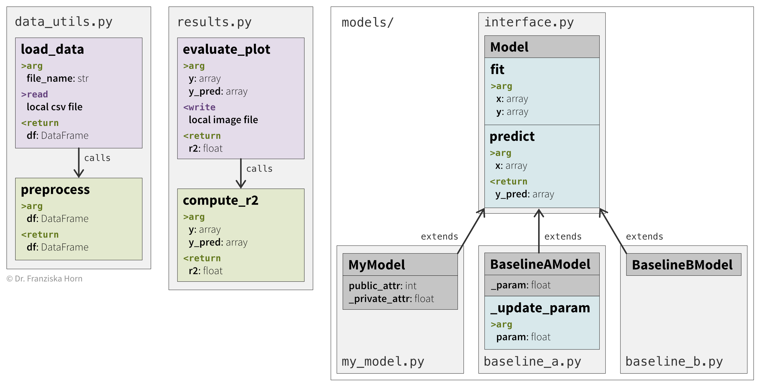
MyModel) that extend another class (Model), only the additional attributes and methods are listed for that class. The arrows indicate dependencies.
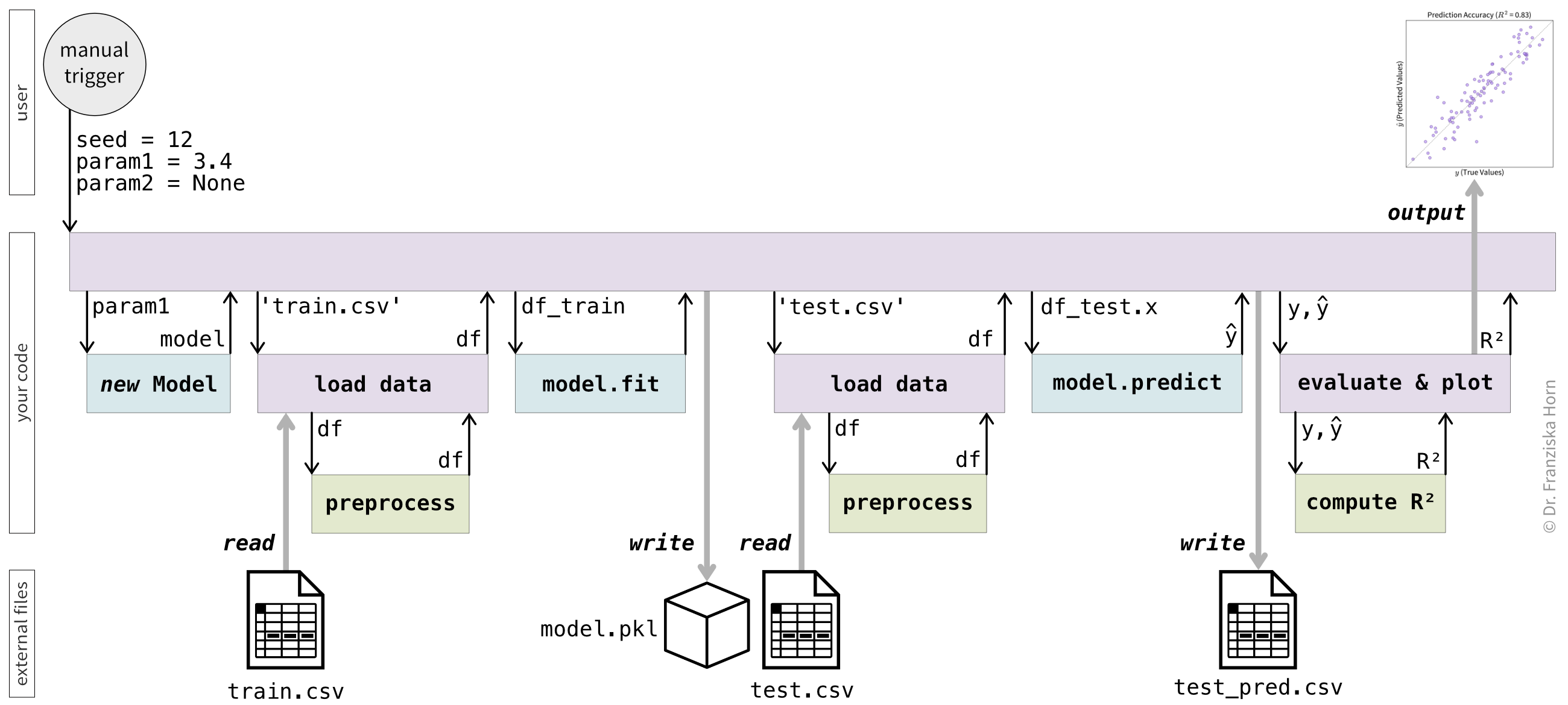
Behavior: Mapping Out Your Script
Our second sketch outlines the script you’ll execute to create the results you want, which builds upon the components from your personal library (Figure 4.16). When designing the flow of your script, consider:
- How the script is triggered – Does it take command-line arguments? What inputs does it require?
- What the final output should be – A results plot? A summary table? Something else?
- Which intermediate results should be saved – If your script crashes, you don’t want to start over. Since variables in memory disappear when the script terminates, consider saving key outputs to disk at logical checkpoints.
- Which functions and classes from your library are used at each step – Also, note any external resources (e.g., files, databases, or APIs) the code interacts with.
At this point, you should have a clear understanding of:
- The inputs and transformations required to produce your desired outputs—what constitutes working code.
- How to structure this code into good code by creating cohesive, decoupled, and reusable units that use simple interfaces to abstract away complicated implementation details.
The fourth Cynefin category is chaotic, where cause and effect are unknowable. In software, this could be compared to rare cosmic-ray-induced bit flips that cause random, unpredictable behavior.↩︎
In some programming languages, you can define constants—variables whose values cannot be changed. These are often declared as global variables so that all other code can reference the same value. In Python, constants are defined by convention using
ALL_CAPSvariable names. However, Python does not enforce immutability, so the value can still be changed despite the naming convention.↩︎The
__init__.pyfile is needed to turn a directory into a package from which other scripts can import functionality. Usually, the file is completely empty.↩︎