A Practitioner’s Guide to Machine Learning

Different types of models

The most important task of a data scientist is to select an appropriate model (and its hyperparameters) for solving a problem.

Three considerations when choosing a supervised learning model

1. Problem type: What kind of problem are you trying to solve: regression or classification?
→ Depends on the type of target variable, i.e., if it has continuous or discrete values.
2. Problem complexity: How complicated is the relationship between the input features and target variable: linear or nonlinear?
→ Depends on the available data, i.e., how easily the target can be predicted from the inputs.
3. Algorithmic approach: Which type of model works best for this dataset size & complexity: features-based or similarity-based?
→ Depends on the model you choose, i.e., it either learns according to the first or second strategy.

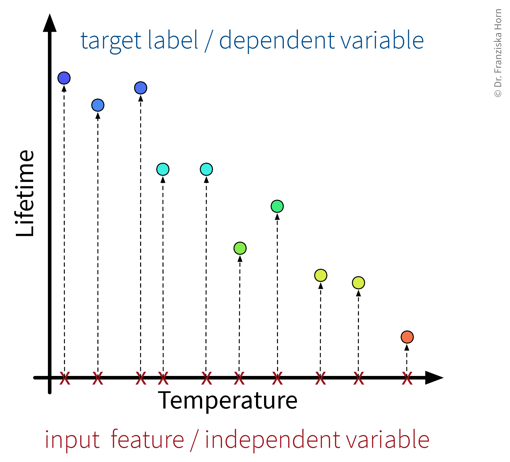
Problem type: regression vs. classification

The type of the target variable that we want to predict determines whether we are dealing with a regression or classification problem.

Regression

Prediction of continuous value(s) (e.g., price, number of users, etc.).

Classification

Prediction of discrete values:

binary (e.g., product will be faulty: yes/no)
multi-class (e.g., picture displays cat/dog/house/car/…)
multi-label (e.g., picture may display multiple objects)

→ Many classification models actually predict probabilities for the different classes, i.e., a score between 0 and 1 for each class. The final class label is then chosen by applying a threshold on this score (typically 0.5 for binary classification problems) or by taking the outcome with the highest score (in multi-class problems).

⇒ Whether we are dealing with a regression or classification problem is important to know and has implications for our overall workflow, e.g., how we define & measure success. However, the actual models that we use to solve these problems are very similar, e.g., almost all sklearn models exist in either a Regressor or Classifier variant to generate the appropriate output for the respective problem type.

In some cases it is even entirely up to us whether to frame the task as a regression or classification problem.

Example: A product is deemed faulty, if it breaks within the warranty period of 6 months, where we assume that normally the product would be used at most 300 times during these 6 months.

Depending on the use case, we might either be interested in how long a product lasts in total, or only whether this product will be a warranty case or not, i.e., we could formulate the problem as:

A regression task: Predict, after how many uses the product will break.
A classification task: Predict, if the product will break before it was used 300 times.

However, in many cases with a continuous target variable, we can learn a more accurate prediction model with the regression approach, since here the labels carry more information and edge case errors are not penalized as much. For example, in the classification case, predicting that a product is okay when it lasted 299 uses would be just as wrong as predicting ‘okay’ for a product that lasted only 2 uses.
If the workflow, where our model is later embedded in, requires a classification output, we can still transform the regression output of the model into a classification output later by simply setting a threshold, i.e., in this case if the regression model predicts a value lower than 300 we would output ‘faulty’ and otherwise ‘okay’.

Problem complexity: linear or nonlinear

In accordance with the product warranty example described above, we now illustrate what it means for a problem to be linear or nonlinear on a small toy dataset:

The first input feature we consider is the production temperature, which is an independent variable, since the operator in control of the production process is free to just choose some value here. The target variable that we want to predict is the lifetime of the produced product and is dependent on this input variable. For the different temperature settings that were tested, we have collected the respective lifetime measurements (and, as you can imagine, getting such labels can be quite expensive, since these products not only needed to be produced, but also go through some stress test to determine after how many uses they break).

As you might have already guessed, the relationship between the target variable lifetime and the input feature temperature (top left) is a linear one, i.e., we could describe it by a straight line. Since the lifetime is a continuous variable, this is a regression problem. However, by defining some cutoff on the target variable (e.g., at 300 usages for in and out of warranty), this problem can be transformed into a classification problem, where the task here is to distinguish between faulty and good products (bottom left). Again, the relationship between the target and the input variable temperature is linear, since the problem can be solved by drawing one line parallel to the y-axis, which defines some threshold on the temperature, where all data points with a temperature lower than this threshold would be classified as ‘ok’ and those products produced at a higher temperature would be predicted as ‘broken’. In the center panel, we have the same situation only this time with a different input feature, pressure. In the regression case, the lifetime values now follow some quadratic curve, i.e., we could not adequately describe the relationship between our target variable and the input feature ‘pressure’ with a single straight line, which makes this a nonlinear problem. Similarly, in the classification case below, we would need to define two thresholds on the pressure values to separate the two classes, i.e., again we could not solve the problem with a single straight line. While these four examples were univariate problems, i.e., with a single input variable, in machine learning we usually deal with multivariate problems, often with hundreds or even thousands of input features. For the case of two input variables, this is illustrated on the right, where the data is now plotted in a scatter plot where the axis correspond to the features temperature and pressure, while the color of the dots indicates the target value (either on a continuous scale or the discrete class labels). In the multidimensional case, a problem would be considered linear if it can by solved by a single hyperplane (instead of a line) in the input feature space.

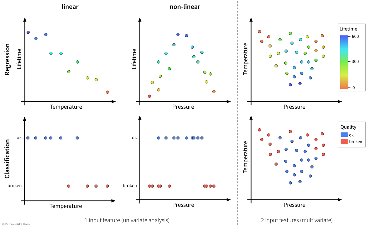
As illustrated in the above examples, whether a problem can be solved by a simple linear model (i.e., a single straight line or hyperplane) or requires a more complex nonlinear model to adequately describe the relationship between the input features and target variable entirely depends on the given data.
This also means that sometimes we can just install an additional sensor to measure some feature that is linearly related to the target variable or do some feature engineering to then be able to get satisfactory results with a linear model, i.e., sometimes, with the right preprocessing, a nonlinear problem can also be transformed into a linear one.

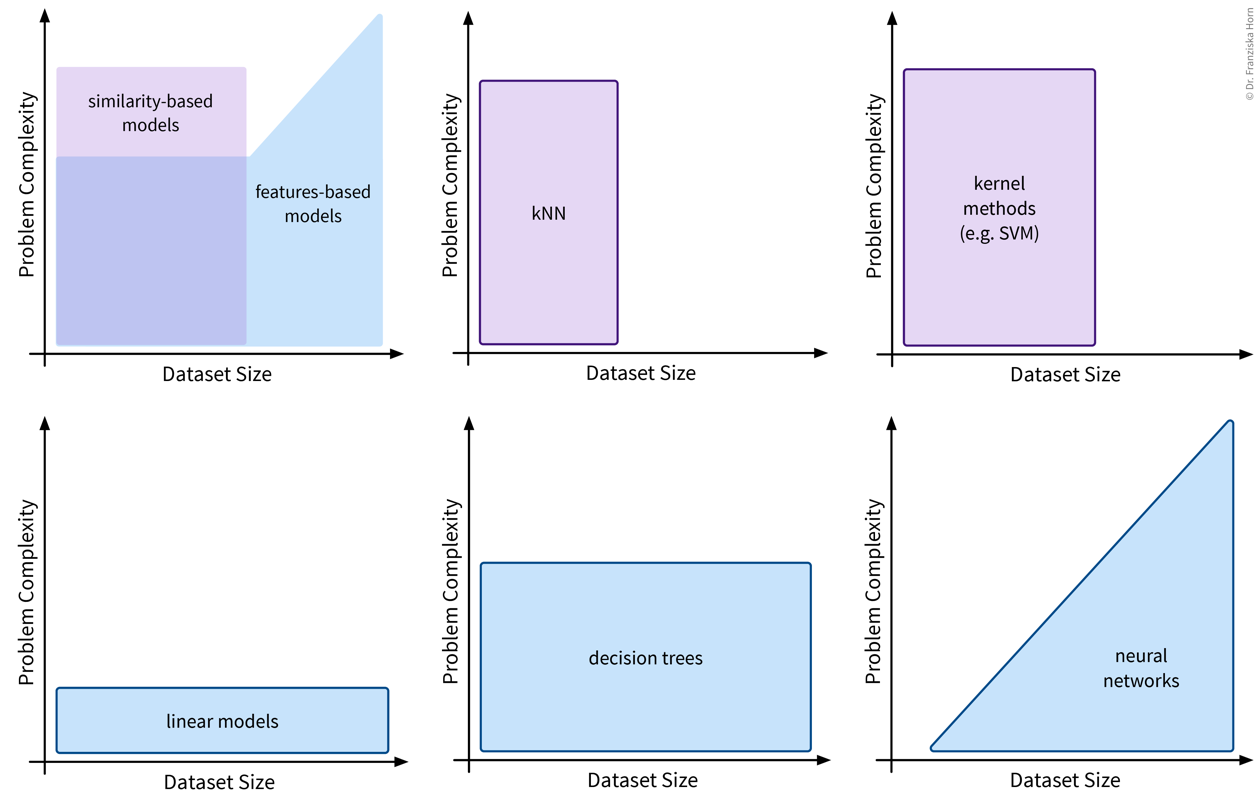
Algorithmic approaches: features-based vs. similarity-based models

Finally, lets look at how the different models work and arrive at their predictions. This is what really distinguishes the various algorithms, whereas we have already established that there always exists a regression and a classification variant of each model and some models are inherently expressive enough that they can be used to describe nonlinear relationships in the data, while others will only yield satisfactory results if there exists a linear relationship between the available input features and the target variable.

Features-based models learn some parameters or rules that are applied directly to a new data point’s input feature vector \(\mathbf{x} \in \mathbb{R}^d\). Similarity-based models, on the other hand, first compute a vector \(\mathbf{s} \in \mathbb{R}^n\) with the similarities of the new sample to the training data points and the model then operates on this vector instead of the original input features.

Left: Features-based models are described by a parametrized function that operates on the original input features. For example, in the regression case (top), the predicted target for a new data point is the value on the line corresponding to its input features, while in the classification case (bottom), the prediction is made according to on which side of the dividing line the inputs lie. Right: The similarity-based models make the prediction for a new sample based on this data point’s nearest neighbors. Depending on the type of model, this could be as simple as predicting the average target value of the nearest neighbors (regression, top) or their most frequent class (classification, bottom).

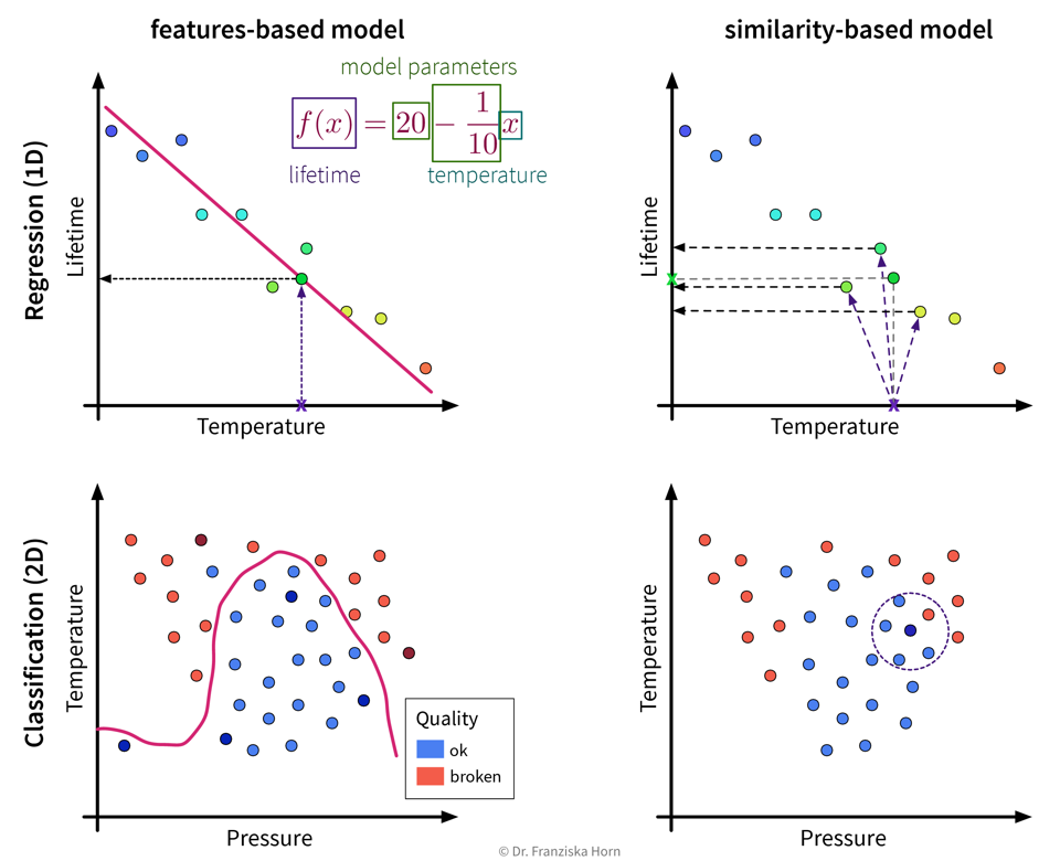
This distinction between algorithmic approaches is not only interesting from a theoretical point of view, but even more so from a practitioner’s perspective: When using a similarity-based algorithm, we have to be deliberate about which features to include when computing the similarities, make sure that these features are appropriately scaled, and in general think about which similarity measure is appropriate for this data. For example, we could capture domain knowledge by using a custom similarity function specifically tailored to the problem. When using a features-based model, on the other hand, the model itself can learn which features are most predictive by assigning individual weights to each input feature and therefore possibly ignore irrelevant features or account for variations in heterogeneous data. But of course, subject matter expertise is still beneficial here, as it can, for example, guide us when engineering additional, more informative input features.

Okay, now, when should we use which approach?

Features-based models

Number of features should be less than the number of samples!
Good for heterogeneous data due to individual feature weights (although scaling is usually still a good idea).
Easier to interpret (since they describe a direct relationship between input features & target).

Similarity-based models

Nonlinear models for small datasets.
Need appropriate similarity function → domain knowledge! (especially for heterogeneous data)

This is an overview of the different features-based and similarity-based models we’ll discuss in the following chapters, as well as for which dataset size and problem complexity they are appropriate: While linear models are rather simple and — as the name suggests — only yield good results for linear problems, they are very efficient and can be applied to large datasets. Decision trees are very efficient as well, but can also capture more complex relationships between inputs and output. Similarity-based models like k-nearest neighbors (kNN) or their more sophisticated cousin kernel methods, on the other hand, can be used to solve very complex nonlinear problems, however, as they require the computation of a similarity matrix that scales with the number of training points, they should only be applied to comparatively small datasets (~ a few thousand points). Finally, neural networks are the most sophisticated model class and can be used to solve extremely complex problems, but they are also rather data hungry (depending on the size of the network).