A Practitioner’s Guide to Machine Learning

Data Preprocessing

Now that we better understand our data and verified that it is (hopefully) of good quality, we can get it ready for our machine learning algorithms.

Raw Data: can come in many different forms, e.g., sensor measurements, pixel values, text (e.g., HTML page), SAP database, …
→ n data points, stored as rows in an excel sheet, as individual files, etc.

What constitutes one data point? It’s always important to be really clear about what one data point actually is, i.e., what the inputs look like and what we want back as a result from the model for each sample / observation. Think of this in terms of how you plan to integrate the ML model with the rest of your workflow: what data is generated in the previous step and can be used as input for the ML part, and what is needed as an output for the following step?

Preprocessing

transforming and enriching the raw data before applying ML, for example:

remove / correct missing or wrongly entered data (e.g., misplaced decimal point)
exclude zero variance features (i.e., variables with always the same value) and nonsensical variables (e.g., IDs)
feature extraction: transform into numerical values (e.g., unstructured data like text)
feature engineering: compute additional/better features from the original variables

⇒ feature matrix \(\,X \in \mathbb{R}^{n\times d}\): n data points; each represented as a d-dimensional vector (i.e., with d features)
Please note that, in general, it is important that all samples in a dataset are represented as the same kind of fixed-length vectors. E.g., if the first position (i.e., feature) in the vector of one sample represents the temperature at which a product was produced, then the first position in the feature vector of another sample can not be this product’s height. This is critical, because most ML models learn some kind of weights that act on the individual features and if these are always at different positions (or missing for some data points), then the algorithm would not be able to apply the correct weight to the respective feature.

Prediction Targets?

→ label vector \(\,\mathbf{y}\) : n-dimensional vector with one target value per data point

What constitutes one data point?

Even given the same raw data, depending on what problem we want to solve, the definition of ‘one data point’ can be quite different. For example, when dealing with time series data, the raw data is in the form ‘n time points with measurements from d sensors’, but depending on the type of question we are trying to answer, the actual feature matrix can look quite different:

1 Data Point = 1 Time Point: e.g., anomaly detection ⇒ determine for each time point if everything is normal or if there is something strange going on:

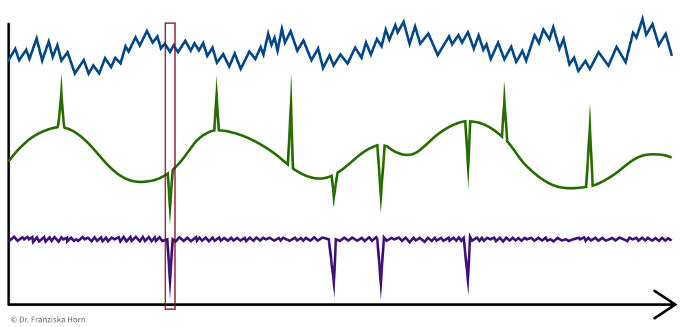
→ \(X\): n time points \(\times\) d sensors, i.e., n data points represented as d-dimensional feature vectors
1 Data Point = 1 Time Series: e.g., cluster sensors ⇒ see if some sensors measure related things:

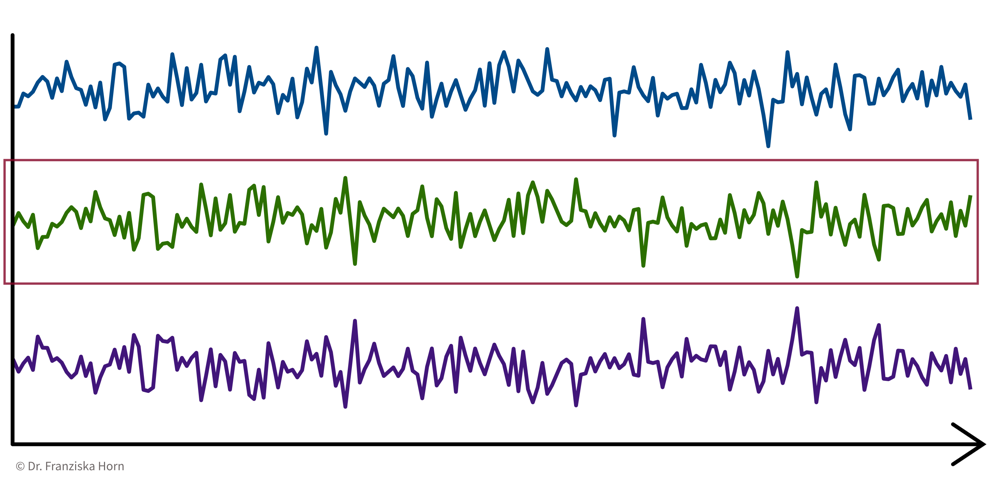
→ \(X\): d sensors \(\times\) n time points, i.e., d data points represented as n-dimensional feature vectors
1 Data Point = 1 Time Interval: e.g., classify time segments ⇒ products are being produced one after another, some take longer to produce than others, and the task is to predict whether a product produced during one time window at the end meets the quality standards, i.e., we’re not interested in the process over time per se, but instead regard each produced product (and therefore each interval) as an independent data point:

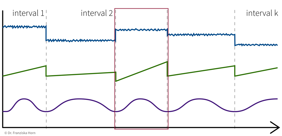
→ Data points always need to be represented as fixed-length feature vectors, where each dimension stands for a specific input variable. Since the intervals here have different lengths, we can’t just represent one product as the concatenation of all the sensor measurements collected during its production time interval, since these vectors would not be comparable for the different products. Instead, we compute features for each time segment by aggregating the sensor measurements over the interval (e.g., min, max, mean, slope, …).
→ \(X\): k intervals \(\times\) q features (derived from the d sensors), i.e., k data points represented as q-dimensional feature vectors

Feature Extraction

Machine learning algorithms only work with numbers. But some data does not consist of numerical values (e.g., text documents) or these numerical values should not be interpreted as such (e.g., sports players have numbers on their jerseys, but these numbers don’t mean anything in a numeric sense, i.e., higher numbers don’t mean the person scored more goals, they are merely IDs).
For the second case, statisticians distinguish between nominal, ordinal, interval, and ratio data, but for simplicity we lump the first two together as categorical data, while the other two are considered meaningful numerical values.

For both text and categorical data we need to extract meaningful numerical features from the original data. We’ll start with categorical data and deal with text data at the end of the section.

Categorical features can be transformed with a one-hot encoding, i.e., by creating dummy variables that enable the model to introduce a different offset for each category.
For example, our dataset could include samples from four product categories circle, triangle, square, and pentagon, where each data point (representing a product) falls into exactly one of these categories. Then we create four features, is_circle, is_triangle, is_square, and is_pentagon, and indicate a data point’s product category using a binary flag, i.e., a value of 1 at the index of the true category and 0 everywhere else:
e.g., product category: triangle ⇒ [0, 1, 0, 0]

from sklearn.preprocessing import OneHotEncoder

Feature Engineering & Transformations

Often it is very helpful to not just use the original features as is, but to compute new, more informative features from them — a common practice called feature engineering. Additionally, one should also check the distributions of the individual variables (e.g., by plotting a histogram) to see if the features are approximately normally distributed (which is an assumption of most ML models).

Generate additional features (i.e., feature engineering)

General purpose library: missing data imputation, categorical encoders, numerical transformations, and much more.
→ feature-engine library
Feature combinations: e.g., product/ratio of two variables. For example, compute a new feature as the ratio of the temperature inside a machine to the temperature outside in the room.
→ autofeat library (Disclaimer: written by yours truly.)
Relational data: e.g., aggregations across tables. For example, in a database one table contains all the customers and another table contains all transactions and we compute a feature that shows the total volume of sales for each customer, i.e., the sum of the transactions grouped by customers.
→ featuretools library
Time series data: e.g., min/max/average over time intervals.
→ tsfresh library

⇒ Domain knowledge is invaluable here — instead of blindly computing hundreds of additional features, ask a subject matter expert which derived values she thinks might be the most helpful for the problem you’re trying to solve!

Aim for normally/uniformly distributed features

This is especially important for heterogeneous data:
For example, given a dataset with different kinds of sensors with different scales, like a temperature that varies between 100 and 500 degrees and a pressure sensor that measures values between 1.1 and 1.8 bar:
→ the ML model only sees the values and does not know about the different units
⇒ a difference of 0.1 for pressure might be more significant than a difference of 10 for the temperature.

for each feature: subtract mean & divide by standard deviation (i.e., transform an arbitrary Gaussian distribution into a normal distribution)
```
from sklearn.preprocessing import StandardScaler
```

for each feature: scale between 0 and 1

from sklearn.preprocessing import MinMaxScaler

map to Gaussian distribution (e.g., take log/sqrt if the feature shows a skewed distribution with a few extremely large values)
```
from sklearn.preprocessing import PowerTransformer
```

Not using (approximately) normally distributed data is a very common mistake!

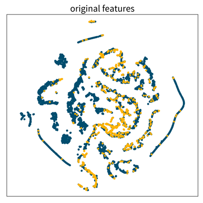
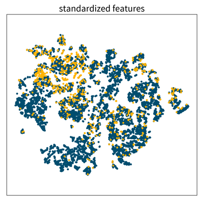
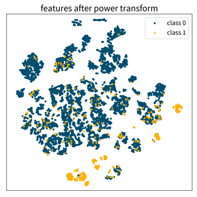
Three 2D visualizations created with the dimensionality reduction method t-SNE of the same dataset, first using the original feature vectors, then on standardized data, and lastly after applying a power transformation. Each dot is one data point where the color denotes the point’s class.

Computing Similarities

Many ML algorithms rely on similarities or distances between data points, computed with measures such as:

Euclidean distance
Cosine similarity (e.g., when working with text data)
Similarity coefficients (e.g., Jaccard index)
… and many more.

from sklearn.metrics.pairwise import ...

Which feature should have how much influence on the similarity between points? → Domain knowledge!

⇒ Scale / normalize heterogeneous data: For example, the pressure difference between 1.1 and 1.3 bar might be more dramatic in the process than the temperature difference between 200 and 220 degrees, but if the distance between data points is computed with the unscaled values, then the difference in temperature completely overshadows the difference in pressure.
⇒ Exclude redundant / strongly correlated features, as they otherwise count twice towards the distance.

Working with Text Data

As mentioned before, machine learning algorithms can not work with text data directly, but we first need to extract meaningful numerical features from it.

Feature extraction: Bag-of-Words (BOW) TF-IDF features:

Represent a document as the weighted counts of the words occurring in the text:

Term Frequency (TF): how often does this word occur in the current text document.
Inverse Document Frequency (IDF): a weight to capture how significant this word is. This is computed by comparing the total number of documents in the dataset to the number of documents in which the word occurs. The IDF weight thereby reduces the overall influence of words that occur in almost all documents (e.g., so-called stopwords like ‘and’, ‘the’, ‘a’, …).

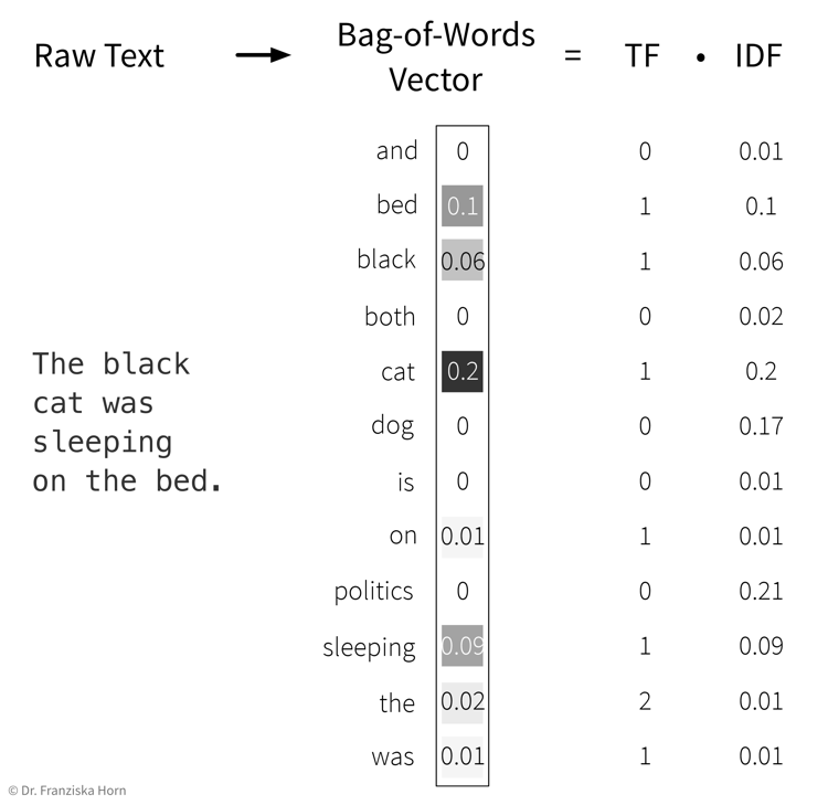Please note that here the feature vector is shown as a column vector, but since each document is one data point, it is actually one row in the feature matrix \(X\), while the TF-IDF values for the individual words are the features in the columns.

→ First, the whole corpus (= a dataset consisting of text documents) is processed once to determine the overall vocabulary (i.e., the unique words occurring in all documents that then make up the dimensionality of the BOW feature vector) and to compute the IDF weights for all words. Then each individual document is processed to compute the final TF-IDF vector by counting the words occurring in the document and multiplying these counts with the respective IDF weights.

from sklearn.feature_extraction.text import TfidfVectorizer

Computing similarities between texts (represented as TF-IDF vectors) with the cosine similarity:: Scalar product (→ linear_kernel) of length normalized TF-IDF vectors:

\[sim(\mathbf{x}_i, \mathbf{x}_j) = \frac{\mathbf{x}_i^\top \mathbf{x}_j}{\|\mathbf{x}_i\| \|\mathbf{x}_j\|} \quad \in [-1, 1]\]

i.e., the cosine of the angle between the length-normalized vectors:

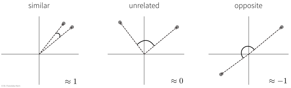
→ similarity score is between [0, 1] for TF-IDF vectors, since all entries in the vectors are positive.

Food for thought: Human vs. TF-IDF + Cosine Similarity understanding

The hotel was great, but the weather was bad.
vs.
The weather was great, but the hotel was bad.
vs.
The accommodation was wonderful, but it was raining all day.

For which of the above sentences would you say that they mean something similar?
Which sentence pairs would be assigned a high or lower similarity score when they are represented as TF-IDF vectors and the similarity is computed with the cosine similarity?

Disadvantages of TF-IDF vectors:

Similarity between individual words (e.g., synonyms) is not captured, since each word has its own distinct dimension in the feature vector and is therefore equally far away from all other words.
Word order is ignored → this is also where the name “bag of words” comes from, i.e., imagine all the words from a document are thrown into a bag and shook and then we just check how often each word occurred in the text.