A Practitioner’s Guide to Machine Learning

Decision Trees

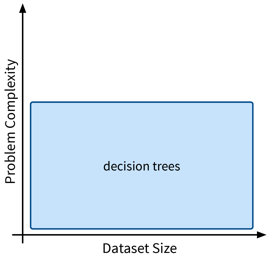
Next, we’ll look at decision trees, another type of features-based model that is very efficient as well, but can also capture more complex relationships between inputs and output.

We’ll describe the decision tree algorithm with the help of an example dataset:

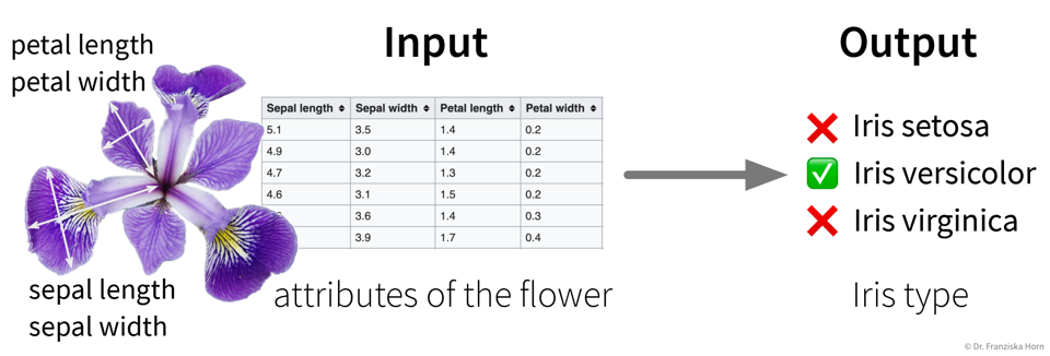
Example: Iris Dataset: The famous Iris dataset was initially studied by the influential statistician R. Fisher. It includes samples from three different types of Iris flowers, each described by four measurements. The task is to classify to which type of Iris flower a sample belongs:

Main idea: Iteratively set a threshold on one of the features such that the remaining samples are split into two “cleaner” groups, where “clean” means that all samples in a group have a similar label, e.g., belong to the same class in case of a classification problem:

Left: Scatter plot of the data, which shows how the splits of the decision tree translate into a decision surface in the feature space, which also shows the characteristic cuts orthogonal to the respective axis (→ new points are classified according to the color of the shaded areas). Right: Illustration of the learned decision tree: Starting left at the root of the tree, the first decision is made to split the data at the ‘petal width’ feature, where all samples with a value smaller than 0.8 are classified as setosa Irises (⇒ perfectly clean group at this leaf) and the other samples advance to a followup decision. In the lower branch of the tree, the remaining samples are now split again according to their petal width and then again at their petal length (it is a coincidence that the same variable is used in both branches at this level to make the cut). Eventually, at each leaf (i.e., terminal node of the tree), the samples that ended up there are mostly from one single class, i.e., the decision tree succeeded in splitting the dataset into cleaner groups. (Please note that decision trees are normally drawn from top to bottom and, unlike real trees, their root is at the top and their branches and leaves grow towards the bottom — the computer scientist who came up with binary trees probably spent too much time indoors…).

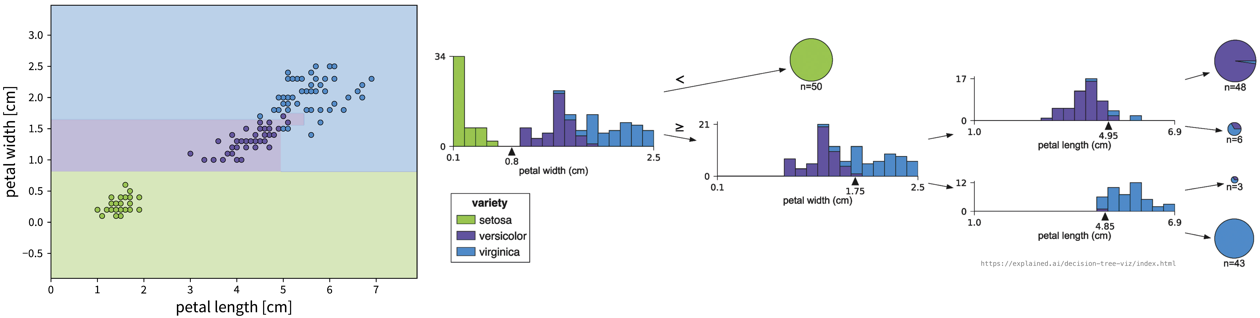
To classify a new sample (i.e., if we went for a walk and found an Iris flower and decided to measure it), we compare the flower’s measurements to the thresholds in the tree (starting at the root) and depending on the leaf we end up in we get a prediction for the Iris type as the most frequent class of the training samples that ended up in this leaf. For regression problems, the tree is built in the same way, but the final prediction is given as the mean of the target variable of the training samples in a leaf.

The decision tree algorithm comes up with the decisions by essentially examining the histograms of all features at each step to figure out for which of the features the distributions for the different classes is separated the most and then sets a threshold there to split the samples.

from sklearn.tree import DecisionTreeClassifier, DecisionTreeRegressor

Important Parameters:

→ max_depth: Maximum number of decisions to make about a sample.
→ min_samples_leaf: How many samples have to end up in each leaf (at least), to prevent overly specific leaves with only a few samples.

Pros

Easy to interpret (i.e., we know exactly what decisions were made to arrive at the prediction).
Good for heterogeneous data: no normalization necessary since all features are considered individually.

Careful

If the hyperparameters (e.g., min_samples_leaf) aren’t set appropriately, it can happen that the tree becomes very specific and memorizes individual samples, which means it probably wont generalize well to new data points (also called “overfitting”, e.g., in the example above, one of the leaves contains only three samples, which might not have been a very useful split).
Unstable: small variations in the data can lead to very different trees.