Linear Models
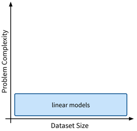
The first type of supervised learning model that we’ll look at in more detail are linear models, which are a type of features-based model that are very efficient (i.e., can be used with large datasets), but, as the name suggests, are only capable of describing linear relationships between the input and target variables.
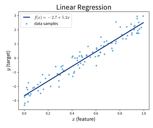
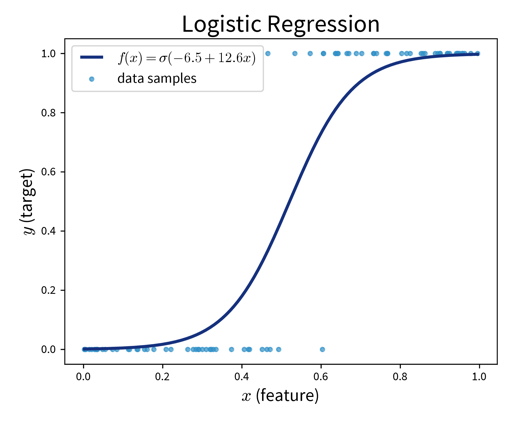
Linear models can be used for regression problems (→ the standard linear regression model that you might have already heard of) as well as for classification problems (→ logistic regression, which predicts a probability score between 0 and 1):
- Main idea
-
Prediction is a linear combination of the input features (and intercept \(b\)):
Linear Regression:
Find \(\mathbf{w}\) that minimizes MSE \(\| \mathbf{y} - \mathbf{\hat y}\|_2^2\) with \(\hat y\) computed as in the formula above.
Logistic Regression (→ for classification problems!):
Make predictions as
where \(\sigma(z)\) is the so-called sigmoid (or logistic) function that squeezes the output of the linear model within the interval \([0, 1\)] (i.e., the S-curve shown in the plot above).
from sklearn.linear_model import LinearRegression, LogisticRegression- Pros
-
-
Linear models are good for small datasets.
-
Extensions for nonlinear problems exist ⇒ feature engineering (e.g., including interaction terms), GAMs, etc.
When a statistician tells you that they did a “polynomial regression” what they really mean is that they did some feature engineering to include new variables like \(x_5^2\) and \(x_2^3x_7\) and then fitted a linear regression model on this extended set of features. This means the model is still linear in the parameters, i.e., the prediction is still a linear combination of the inputs, but some of the inputs are now polynomial terms computed from the original features.
-
- Careful
-
-
Regularization (to keep \(\mathbf{w}\) in check) is often a good idea.
-
Regularization
Motivation: For uncorrelated but noisy data, which model should you choose?
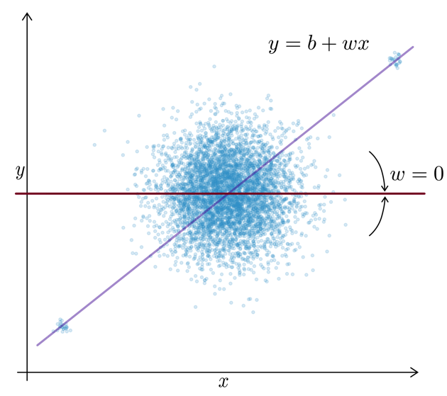
⇒ Regularization = assume no relationship between \(x\) and \(y\) unless the data strongly suggests otherwise.
This is accomplished by imposing constraints on the model’s weights by adding penalty terms in the optimization:
This means the optimal solution now not only achieves a low MSE between the true and predicted values (i.e., the normal linear regression error), but additionally does so with the smallest possible weights. (The regularization therefore also defines a unique solution in the face of collinearity.)
L1 Regularization (→ Lasso Regression): Sparse weights (i.e., many 0, others normal)
→ Good for data with possibly irrelevant features.
L2 Regularization (→ Ridge Regression): Small weights
→ Computationally beneficial; can help for data with outliers.
| When you’re working with a new dataset, it often includes lots of variables, many of which might not be relevant for the prediction problem. In this case, an L1-regularized model is helpful to sort out irrelevant features. Then, when you are sure which input variables are relevant for the prediction problem, an L2-regularized model gives a robust performance. |
from sklearn.linear_model import RidgeCV, LassoLarsCV
Regularization is also used in many other sklearn models. Depending on the type of model (for historical reasons), what we denoted as \(\lambda\) in the formula above is a hyperparameter that is either called alpha or C, where you have to be careful, because while for alpha higher values mean more regularization (i.e., this acts exactly as the \(\lambda\) in the formula above), when the model instead has the hyperparameter C, here higher values mean less regularization!
|
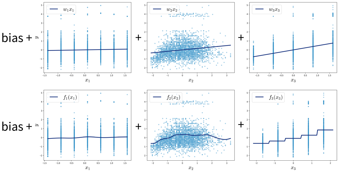
Generalized Additive Models (GAMs)
GAMs are a very powerful generalization of linear models. While in a linear regression, the target variable is modeled as a sum of linear functions of the input variables (parametrized by the respective coefficients), GAMs instead fit a smooth function \(f_k(x_k)\) to each input variable and then predict the target variable as a sum of these: