A Practitioner’s Guide to Machine Learning

Neural Networks

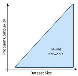
Next up are neural networks (NN), which can be used to solve extremely complex problems (besides regular supervised learning tasks), but that are also rather data hungry (depending on the size of the network).
We’ll only cover the basics here; more advanced NN architectures, like those used to process image and text data, are discussed in the chapter on Deep Learning.

Basic Math

Dangerous Artificial Intelligence

\[\begin{aligned} \begin{pmatrix} W_{11} & W_{12} & \cdots & W_{1j}\\ W_{21} & W_{22} & \cdots & W_{2j}\\ \vdots & \vdots & \ddots & \vdots\\ W_{i1} & W_{i2} & \cdots & W_{ij}\\ \end{pmatrix} \cdot \begin{pmatrix} W_{11} & W_{12} & \cdots & W_{1k}\\ W_{21} & W_{22} & \cdots & W_{2k}\\ \vdots & \vdots & \ddots & \vdots\\ W_{j1} & W_{j2} & \cdots & W_{jk}\\ \end{pmatrix} \cdot \begin{pmatrix} W_{11} & W_{12} & \cdots & W_{1l}\\ W_{21} & W_{22} & \cdots & W_{2l}\\ \vdots & \vdots & \ddots & \vdots\\ W_{k1} & W_{k2} & \cdots & W_{kl}\\ \end{pmatrix} \cdot \begin{pmatrix} W_{11} & W_{12} & \cdots & W_{1m}\\ W_{21} & W_{22} & \cdots & W_{2m}\\ \vdots & \vdots & \ddots & \vdots\\ W_{l1} & W_{l2} & \cdots & W_{lm}\\ \end{pmatrix} \end{aligned}\]

Deep learning just means using more matrices.

Overview

Recap: Linear Models: Prediction is a linear combination of input features (and intercept / bias term \(b\)):

\[f(\mathbf{x}; \mathbf{w}) = b + \langle\mathbf{w},\mathbf{x}\rangle = b + \sum_{k=1}^d w_k \cdot x_k = \hat{y}\]

In the case of multiple outputs \(\mathbf{y}\) (e.g., in a multi-class classification problem \(\mathbf{y}\) could contain the probabilities for all classes):

\[f(\mathbf{x}; W) = \mathbf{x^\top}W = \mathbf{\hat{y}}\]

For simplicity, we omit the bias term \(b\) here; using a bias term is equivalent to including an additional input feature that is always 1.
Intuitive Explanation of Neural Networks: [Adapted from: “AI for everyone” by Andrew Ng (coursera.org)]

Let’s say we have an online shop and are trying to predict how much of a product we will sell in the next month. The price we are willing to sell the product for will obviously influence the demand, as people are trying to get a good deal, i.e., the lower the price, the higher the demand; a negative correlation that can be captured by a linear model. However, the demand will never be below zero (i.e., when the price is very high, people wont suddenly return the product), so we need to adapt the model such that the predicted output is never negative. This can be achieved by applying the max function, in this context also called a nonlinear activation function, to the output of the linear model, so that now when the linear model would return a negative value, we instead predict 0.

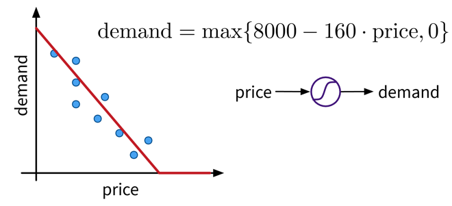A very simple linear model with one input and one output variable and a nonlinear activation function (the max function).

This functional relationship can be visualized as a circle with one input (price) and one output (demand), where the S-curve in the circle indicates that a nonlinear activation function is applied to the result. We will later see these circles as single units or “neurons” of a neural network.

To get better results, we can extend the model and use multiple input features for the prediction:

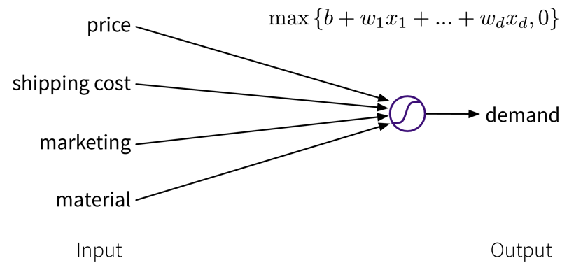A linear model with multiple inputs, where the prediction is computed as a weighted sum of the inputs, together with the max function to prevent negative values.

To improve the performance even further, we could now manually construct more informative features from the original inputs by combining them in meaningful ways (→ feature engineering) before computing the output:

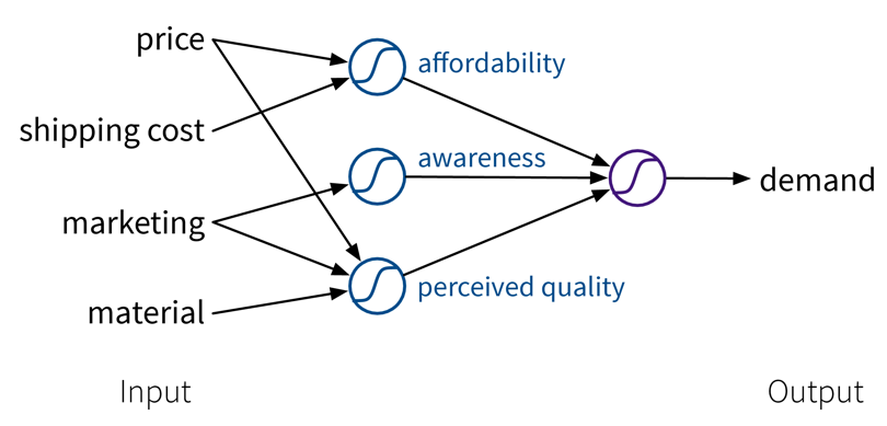Our example is about an online shop, so the customers additionally have to pay shipping fees, which means to reflect the true affordability of the product, we need to combine the product price with the shipping costs. Next, the customers are interested in high quality products. However, not only the actual quality of the raw materials we used to make the product influences how the customers perceive the product, but we can also reinforce the impression that the product is of high quality with a marketing campaign. Furthermore, a high price also suggests that the product is superior. This means by creating these additional features, the price can actually contribute in two ways towards the final prediction: while, on the one hand, a lower price is beneficial for the affordability of the product, a higher price, on the other hand, results in a larger perceived quality.

While in this toy example, it was possible to construct such features manually, the nice thing about neural networks is that they do exactly that automatically: By using multiple layers, i.e., stacking multiple linear models (with nonlinear activation functions) on top of each other, it is possible to create more and more complex combinations of the original input features, which can improve the performance of the model. The more layers the network uses, i.e., the “deeper” it is, the more complex the resulting feature representations.

Since different tasks and especially different types of input data benefit from different feature representations, there exist different types of neural network architectures to accommodate this, e.g.

→ Feed Forward Neural Networks (FFNNs), also called Multi-Layer Perceptrons (MLPs), for ‘normal’ (e.g., structured) data
→ Convolutional Neural Networks (CNNs) for images
→ Recurrent Neural Networks (RNNs) for sequential data like text or time series

We’ll only cover FFNNs here; the other architectures are discussed in the chapter on Deep Learning.

Pros

State-of-the-art performance (especially on data with input invariances).
Prediction for new test points is fast (just a few matrix multiplications).

Careful

Can take a long time to train (use a GPU!!! (or TPU)).
Need a lot of data (depending on the size of the NN architecture).
Solution only a local optimum (which is usually not too problematic in practice, as there are many good optima).
Tricky to train: Performance depends on many parameters like learning rate, batch size, and even the random seed used when initializing the weights!

Feed Forward Neural Network (FFNN)

This is the original and most straightforward neural network architecture, which we’ve already seen in the initial example, only that in practice such a model usually has a few more layers and units per layer. Each layer here is basically a linear model, i.e., it consists of a weight matrix \(W_i\) and some nonlinear activation function \(\sigma_i\) that is applied to the output. These layers are applied sequentially to the input features \(\mathbf{x}\), i.e., the network computes a composite function (in this case for three layers):

\[f(\mathbf{x}) = \sigma_3(\sigma_2(\sigma_1(\mathbf{x^\top}W_1)W_2)W_3) = \mathbf{\hat{y}}\]

Feed Forward Neural Network (FFNN) architecture: The input feature vector \(\mathbf{x}\), representing one data point, is multiplied by the first weight matrix \(W_1\) to create a new vector, which, after applying the nonlinear activation function (e.g., the max function as we’ve seen in the initial example) results in the first hidden layer representation \(\mathbf{x}'\). This new vector is then multiplied by the second weight matrix \(W_2\) and again a nonlinear activation function is applied to yield the second hidden layer representation of the sample, \(\mathbf{x}''\). Depending on how many layers the network has (i.e., how deep it is), this could be repeated multiple times now until finally the last layer computes the predicted output \(\mathbf{\hat{y}}\). While the network is trained, these predicted outputs gets closer and closer to the true outputs for the training samples.

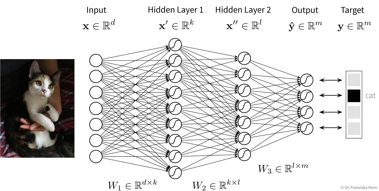
For a regression problem, the output of the network would be a direct prediction of the target values (i.e., without applying a final nonlinear activation function), while for a classification problem, the output consists of a vector with probabilities for the different classes, created by applying a softmax activation function on the output, which ensures all values are between 0 and 1 and sum up to 1.

Test your understanding

Why do we need the nonlinear activation functions between the layers, i.e., how could we simplify a network with multiple layers, if it didn’t have any nonlinear activation functions between the layers?
In what way could we manipulate the parameters (i.e., weight matrices) of an existing neural network without changing its predictions? (This is also a reason why there exist many equally good local optima.)

Number of hidden layers and units:: While the size of the input and output layers are determined by the number of input features and targets respectively, the dimensionality and number of hidden layers of the network is up to us. Usually, the hidden layers get smaller (i.e., have fewer units) as the data moves from the input to the output layer and when experimenting with different settings we can start with no hidden layers (which should give the same result as a linear model) and then progressively increase the size of the network until the performance stops improving. Just play around a bit.

Training Neural Networks: To train a neural network, we first need to choose a loss function that should be optimized (e.g., mean squared error for regression problems or cross-entropy for classification problems).

While for a linear regression model, the optimal weights can be found analytically by setting the derivative of this loss function to 0 and solving for the weights, in a network with multiple layers and therefore many more weights, this is not feasible. Instead, the weights are tuned iteratively using a gradient descent procedure, where the derivative of the loss function w.r.t. each layer is computed step by step using the chain rule by basically pushing the error backwards through the network (i.e., from the output, where the error is computed, to the input layer), also called error backpropagation. At the beginning, all weight matrices are randomly initialized, so, for example, for a classification problem, for a given sample the network would predict approximately equal probabilities for all classes. The weights are then adapted according to their gradient, such that the next time the same samples are passed through the network, the prediction will be closer to the true output (and the value of the loss function is closer to a local minima).

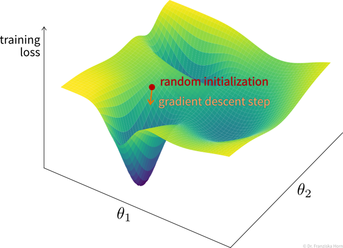Training loss surface over the network’s parameter space (simplified, i.e., showing only two weights (\(\theta_1\) and \(\theta_2\)), while in reality, this would be a super complex nonlinear function in a very high-dimensional space), where every possible weight configuration of a network results in a different loss on the training set. By taking a step into the direction of steepest descent of this loss function, the weights of the network get closer to a configuration where the loss is at a local minimum.

Typically, the weights are adapted over multiple epochs, where one epoch means going over the whole training set once. By plotting the learning curves, i.e., the training and validation loss against the number of training epochs, we can check whether the training was successful (i.e., whether the weights have converged to a good solution).

Since a training set usually contains lots of data points, it would be too computationally expensive to do gradient descent based on the whole dataset at once in each epoch, so we instead use mini-batches, i.e., subsets of usually 16-128 data points, for each training step.

Tips & Tricks

Scale the data (for classification tasks only inputs, for regression tasks also outputs or adapt the bias of the last layer; StandardScaler is usually a good choice) as otherwise the weights have to move far from their initialization to scale the data for us.
Use sample weights for classification problems with unequal class distributions.
NN are trained with gradient descent, which requires a good learning rate (i.e., step size for each training iteration → not too small, otherwise nothing is learned, not too big, otherwise it spirals out of control):

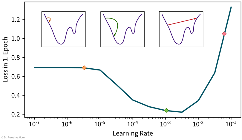A simple strategy to select a suitable initial learning rate is to train the network with different learning rates for one epoch on a subsample of the dataset and then check the loss after training. For too small learning rates (left), the loss will stay the same, while for too large learning rates (right) the loss will be higher after training.
Sanity check: A linear network (i.e., a FFNN with only one layer mapping directly from the inputs to the outputs) should achieve approximately the same performance as the corresponding linear model from sklearn.
Gradually make the network more complex until it can perfectly memorize a small training dataset (to get a network that has enough capacity to at least in principle capture the complexity of the task).
When selecting hyperparameters, always check if there is a clear trend towards an optimal setting; if the pattern seems random, initialize the network with different random seeds to see how robust the results are.
Using a learning rate scheduler (to decrease the learning rate over time to facilitate convergence) or early stopping (i.e., stopping the training when the performance on the validation set stops improving) can improve the generalization performance.
But often it is more important to train the network long enough, like, for hundreds of epochs (depending on the dataset size).

→ more tips for training NN: http://karpathy.github.io/2019/04/25/recipe/