A Practitioner’s Guide to Machine Learning

Kernel Methods

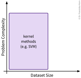
Kernel methods are more sophisticated similarity-based models and were the hot stuff in the late 90s, when datasets were still of moderate size and computers weren’t fast enough to train large neural networks. They have some elegant math behind them, but please don’t be discouraged, if you don’t fully understand it the first time you read it — this is completely normal 😉.

Main idea / “Kernel Trick”: By working on similarities (computed with special kernel functions) instead of the original features, linear methods can be applied to solve nonlinear problems.

Assume there exists some function \(\phi(\mathbf{x})\) (also called a ‘feature map’) with which the input data can be transformed in such a way that the problem can be solved with a linear method (basically the ideal outcome of feature engineering).
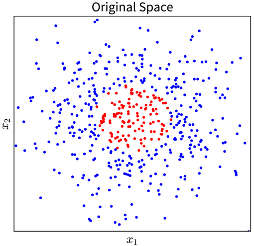
For example, in the simple toy dataset shown below, the two classes become linearly separable when projecting the original input features into the space of their second order monomials:

→ \(\phi(\mathbf{x})\) →
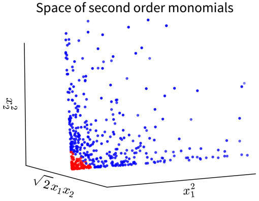
In the original 2D representation on the left, we need a circle (i.e., a nonlinear function) to separate the blue from the red points, while in the 3D plot on the right, the data points are arranged in a cone shape, where we can cut off the red points at the tip of the cone with a hyperplane.

Of course, coming up with such a feature map \(\phi(\mathbf{x})\), especially for more complex problems, isn’t exactly easy. But as you will see, we don’t actually need to know what this transformation looks like!

Example: Kernel Ridge Regression

Remember: In a linear regression model, the prediction for a new data point \(\mathbf{x}'\) is computed as the scalar product of the feature vector with the weight vector \(\mathbf{w}\):

\[\hat{y}' = \mathbf{x}' \mathbf{w}\]

(for simplicity, we omit the bias term here; using a bias term is equivalent to including an additional input feature that is always 1).

The parameters of a linear ridge regression model are found by taking the derivative of the objective function,

\[\| \mathbf{y} - \mathbf{Xw}\|_2^2 + \lambda \| \mathbf{w}\|_2^2\]

with respect to \(\mathbf{w}\), setting it to 0, and solving for \(\mathbf{w}\) (i.e. to find the minimum). This gives the following solution:

\[\mathbf{w} = (\mathbf{X}^\top \mathbf{X} +\lambda I)^{-1}\mathbf{X}^\top \mathbf{y}\]

where \(\mathbf{X} \in \mathbb{R}^{n \times d}\) is the feature matrix of the training data and \(\mathbf{y} \in \mathbb{R}^n\) are the corresponding target values.

Now we replace every occurrence of the original input features \(\mathbf{x}\) in the formulas with the respective feature map \(\phi(\mathbf{x})\) and do some linear algebra:

\[\begin{aligned} \hat{y}' &= \phi(\mathbf{x}') \mathbf{w} \quad\quad\quad\text{ with }\; \mathbf{w} = (\phi(\mathbf{X})^\top \phi(\mathbf{X}) +\lambda I)^{-1}\phi(\mathbf{X})^\top \mathbf{y}\\ &= \phi(\mathbf{x}') (\phi(\mathbf{X})^\top \phi(\mathbf{X}) +\lambda I)^{-1}\phi(\mathbf{X})^\top \mathbf{y}\\ & \quad\quad\vdots\\ &= \underbrace{\phi(\mathbf{x}')\phi(\mathbf{X})^\top}_{\mathbf{k}'= k(\mathbf{x'}, \mathbf{X})} (\underbrace{\phi(\mathbf{X}) \phi(\mathbf{X})^\top}_{\mathbf{K} = k(\mathbf{X}, \mathbf{X})} +\lambda I)^{-1} \mathbf{y}\\ &= \mathbf{k}'\underbrace{(\mathbf{K} +\lambda I)^{-1} \mathbf{y}}_{\mathbf{\alpha}} = \sum_{i=1}^n k(\mathbf{x}', \mathbf{x}_i) \alpha_i \end{aligned}\]

After the reformulation, every \(\phi(\mathbf{x})\) only occurs in scalar products with other \(\phi(\mathbf{x})\), and all these scalar products were replaced with a so-called kernel function \(k(\mathbf{x}', \mathbf{x})\), where \(k(\mathbf{X}, \mathbf{X}) = \mathbf{K} \in \mathbb{R}^{n \times n}\) is the kernel matrix, i.e., the similarity of all training points to themselves, and \(k(\mathbf{x}', \mathbf{X}) = \mathbf{k}' \in \mathbb{R}^{n}\) is the kernel map, i.e., the similarities of the new data point to all training points.

The prediction \(\hat{y}'\) is now computed as a weighted sum of the similarities in the kernel map, i.e., while in the normal linear regression model the sum goes over the number of input features d and the weight vector is denoted as \(\mathbf{w}\), here the sum goes over the number of data points n and the weight vector is called \(\mathbf{\alpha}\).

Kernel Functions \(k(\mathbf{x}', \mathbf{x})\)

A kernel function is basically a similarity function, but with the special requirement that the similarity matrix computed using this function, also called the kernel matrix, is positive semi-definite, i.e., has only eigenvalues \(\geq 0\).

There exist different kinds of kernel functions and depending on how they are computed, they induce a different kind of kernel feature space \(\phi(\mathbf{x})\), where computing the kernel function for two points is equivalent to computing the scalar product of their vectors in this kernel feature space.

We illustrate this on the initial example, where the data was projected into the space of second order monomials. When we compute the scalar product between the feature maps of two vectors \(\mathbf{a}\) and \(\mathbf{b}\), we arrive at a polynomial kernel of second degree:

\[\langle\phi(\mathbf{a}), \phi(\mathbf{b})\rangle = (a_1^2, \sqrt{2}a_1a_2, a_2^2)(b_1^2, \sqrt{2}b_1b_2, b_2^2)^\top = \langle\mathbf{a}, \mathbf{b}\rangle^2 =: k(\mathbf{a}, \mathbf{b})\]

i.e, computing the kernel function \(k(\mathbf{a}, \mathbf{b}) = \langle\mathbf{a}, \mathbf{b}\rangle^2\) between the two points is the same as computing the scalar product of the two feature maps \(\langle\phi(\mathbf{a}), \phi(\mathbf{b})\rangle\).

While for the polynomial kernel of second degree, \(\langle\mathbf{a}, \mathbf{b}\rangle^2\), we could easily figure out that the feature map consisted of the second order monomials, for other kernel functions, the corresponding feature map is not that easy to identify and the kernel feature space might even be infinite dimensional. However, since all the feature map terms \(\phi(\mathbf{x})\) in the kernel ridge regression formulas only occurred in scalar products, we were able to replace them by a kernel function, which we can compute using the original input feature vectors. Therefore, we don’t actually need to know what the respective feature map looks like for other kernel functions!
So while kernel methods are internally working in this really awesome kernel feature space \(\phi(\mathbf{x})\), induced by the respective kernel function, where all our problems are linear, all we need to know is how to compute the kernel function using the original feature vectors.

If you are curious what the kernel feature space looks like for some kernel function, you can use kernel PCA to get an approximation of \(\phi(\mathbf{x})\). Kernel PCA computes the eigendecomposition of a given kernel matrix, thereby generating a new representation of the data such that the scalar product of these new vectors approximates the kernel matrix. This means the new kernel PCA feature vector computed for some data point \(i\) approximates \(\phi(\mathbf{x}_i)\) — however, this still doesn’t tell us what the function \(\phi\) itself looks like, i.e., how to get from \(\mathbf{x}\) to \(\phi(\mathbf{x})\), we only get (an approximation of) the final result \(\phi(\mathbf{x})\).

In the example above you were already introduced to the polynomial kernel of second degree; the generalization, i.e., the polynomial kernel of degree k, is computed as \(\langle\mathbf{x}', \mathbf{x}_i\rangle^k\).

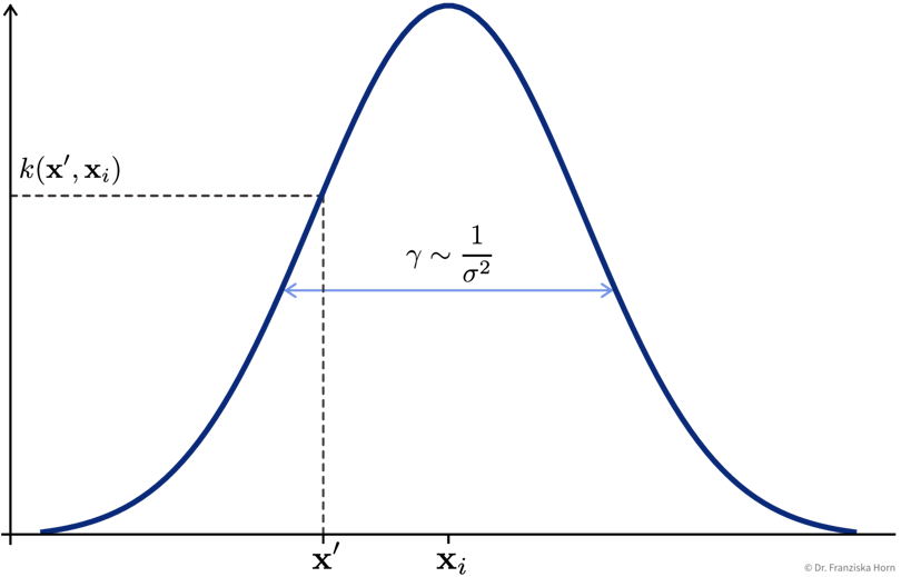
The most popular kernel function that works well in many use cases is the Radial Basis Function (RBF) / Gaussian kernel:

\[k(\mathbf{x}', \mathbf{x}_i) = e^{-\gamma \|\mathbf{x}_i - \mathbf{x}' \|^2}\]

With the RBF kernel function, the similarity of a new point \(\mathbf{x}'\) to the training sample \(\mathbf{x}_i\) is computed by centering a Gaussian function (with a width inversely proportional to \(\gamma\)) over the \(i^{th}\) training sample and then checking where the new point falls on this curve. Depending on the choice of \(\gamma\), either many samples will later contribute to the prediction (if the Gaussian function is very wide and therefore the similarity to multiple training points is large) or only the closest points will be considered (if the curve is very narrow and therefore the similarity to most training examples is close to 0).

Support Vector Machine (SVM): A more efficient method, especially when the training set is large.
Key idea: Only compute similarity to ‘most informative’ training points (= support vectors):

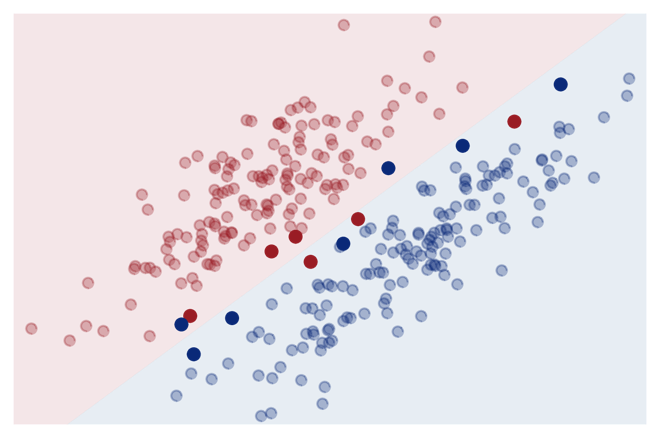
\[\sum_{i=1}^n k(\mathbf{x}', \mathbf{x}_i) \alpha_i \quad \Rightarrow \quad \sum_{i \in \{\text{SV}\}} k(\mathbf{x}', \mathbf{x}_i) \alpha_i\]

This reduces the memory requirements and makes the prediction for new data points much faster, since it is only necessary to store the support vectors and compute the similarity to them instead of the whole training set.

from sklearn.decomposition import KernelPCA     # Kernel variant of PCA
from sklearn.kernel_ridge import KernelRidge    # Kernel variant of ridge regression (-> use SVR instead)
from sklearn.svm import SVC, SVR                # SVM for classification (C) and regression (R)

Important Parameters:

→ kernel: The kernel function used to compute the similarities between the points (→ see sklearn.metrics.pairwise; usually 'rbf').
→ Additionally: Kernel parameters, e.g., gamma for 'rbf' kernel.

Pros

Nonlinear predictions with global optimum.
Fast to train (on medium size datasets; compared to, e.g., neural networks).

Careful

Computationally expensive for large datasets (kernel matrix: \(\mathcal{O}(n^2)\)).
Kernel functions, just like other similarity functions, benefit from scaled heterogeneous data.