A Practitioner’s Guide to Machine Learning

Explainability & Interpretable ML

Explainability is essential to trust a model’s predictions, especially in performance-critical areas like medicine (e.g., diagnosis from x-ray images).

Explainable/Interpretable ML – distinguish between:

Local Explainability: explain individual predictions.
→ Which features from one particular sample swayed the model to make a certain prediction? This can, for example, be visualized as a heatmap like that over the image of a horse, where the classification decision was made mostly because of the copyright notice.
Global Explainability: explain the model behavior in general.
→ Which features are most important over all?

→ Some models are intrinsically interpretable (e.g., linear models, decision trees), others require model-agnostic methods to make them explainable, i.e., for these models the interpretability does not come for free.

Explaining a model and its predictions helps to understand what it learned from the data and why it makes certain mistakes. But only when the model has a good predictive performance and there is reason to believe that the model actually captured the true causal relationship between the inputs and targets, then these explanations might shed light on the true root causes of the underlying process as well. Always discuss the results with a subject matter expert!

Careful

Correlated features can lead to misrepresented feature importances! For example, when using a random forest, one decision tree might use one feature in the root node, while another decision tree uses a second feature that is correlated with the first, which means that overall it seems that both features are only somewhat important, while in fact they are just interchangeable and therefore their true feature importance would be the sum of the two individual feature importances.
Beware of Simpson’s paradox.
Possibly look at results for different subsamples of the data.
Compare feature importances obtained for different models to get a better feeling for which features truly matter for the problem, e.g., investigate why a linear model and a decision tree might base their decisions on different features.

Recommended Reading: Interpretable ML Book, which additionally covers some more advanced methods. However, please keep in mind that explainable AI is about understanding better what happens — if you use a complex method to explain a model (e.g., the popular SHAP values) where it is difficult to understand how the explanations were derived, then this might instead result in further uncertainty.

Explaining Decision Trees (& Random Forests)

Explaining individual predictions: retrace decision path (in a single tree).

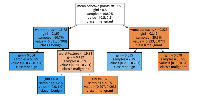
This is an example of a decision tree plot generated with sklearn. The decision tree has its root at the top (where we start when predicting for a new sample) and the leaves (i.e., those nodes that don’t branch off anymore) at the bottom (where we stop and make the final prediction). Each node in the tree shows in the first line the variable based on which the next split is made incl. the threshold value (except for leaf nodes), then the current Gini impurity (i.e., how homogeneous the labels of all the samples that ended up in this node are; this is what the decision tree internally optimizes, i.e., notice how the value gets smaller on at least one side after a split), then the fraction of samples that ended up in this node, and the distribution of samples for the different classes (for a classification problem), as well as the label that would be predicted for a sample at this point. So when making a prediction for a new sample with a decision tree, we start at the root node of the tree and then follow the branches down depending on the sample’s feature values until we reach a leaf node and would then know exactly based on which feature thresholds the prediction for the sample was made.

Global interpretation: a trained decision tree or random forest has an attribute feature_importances_, which indicates how much each feature contributed to reducing the (Gini) impurity. This is related to the position of the feature in the tree and how many samples pass through the respective node.

This is just a bar plot of the values from the feature_importances_ attribute of the decision tree shown above. When we’re using a random forest instead of a single decision tree, it would be impractical to plot all of the individual trees contained in the forest to explain individual predictions, but a random forest at least also has the feature_importances_ attribute to examine the global importance of the different features.

Explaining Linear Models (& Neural Networks)

Since the formula used to make predictions with a linear model is very simple, we can easily understand what is going on. To assess the importance of individual features, either for a single sample or overall, the sum can be decomposed into its individual components:
\(\hat{y} = b + \sum_{k=1}^d w_k \cdot x_k\) ⇒ effect of feature k for ith data point: \(w_k \cdot x_k^{(i)}\):

The feature effects for a single sample are indicated by the red crosses, i.e., these show whether each feature contributed positively or negatively (or not at all) to the final prediction for this one sample. By computing the feature effects for all samples, we can generate the box plots shown below the red crosses, which display the distribution of feature effects for all samples and therefore indicate which features are overall important for the prediction (= those with the largest absolute values). For example, in this plot we can see that the feature 'AveOccup' has an effect of around zero for all but one sample, which indicates that the model might have overfit on one outlier point and it might be best to exclude this feature altogether.

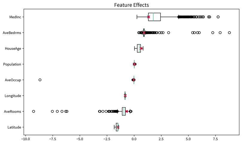
→ It is easier to understand and validate the results if only a few features are considered important. Use an L1-regularized model (e.g., linear_model.LassoLarsCV) to get sparse weights.

Generalization for neural networks: Layer-wise Relevance Propagation (LRP): Similar to how the prediction of the linear model was split up into the contributions of the individual input features, by keeping track of the gradients in a neural network, the decision can be decomposed as well to obtain the influence of each feature on the final prediction. This is similar to what happens in the backpropagation procedure when training the network, only that with LRP not the prediction error, but the prediction itself is propagated backwards layer by layer (hence the name) until we arrive at the input layer and get the individual contributions of the features.
For torch networks, this approach is implemented in the captum library as the ‘Input X Gradient’ method. The library also contains many other methods for interpreting neural networks, however, I find this the most natural approach, since it is a direct extension of the intuitive feature effects approach used to interpret linear models.

[Global] Model-agnostic: permutation feature importance

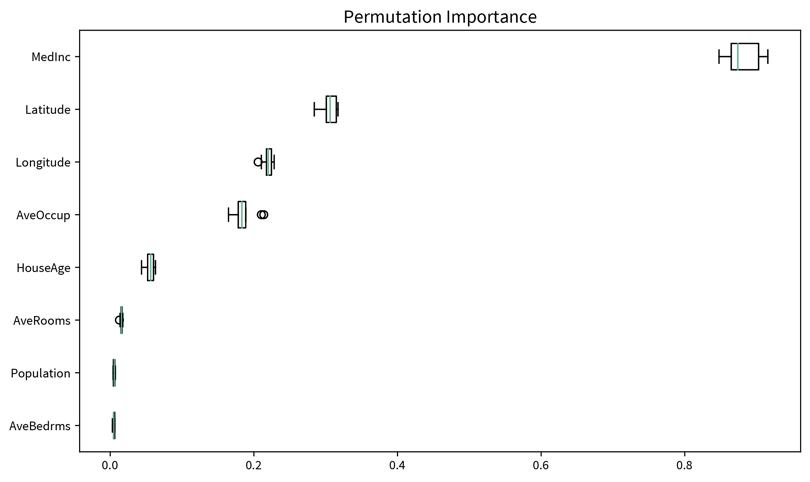
The first question when it comes to global explainability is always “Which features are important?”, i.e., how much does the model rely on each feature when making its predictions? We can shed light on this using the permutation importance, which, for each feature, is computed like this:

‘Feature importance’ = ‘performance of trained model on original dataset’ minus ‘performance when values for this feature are shuffled’.

I.e., first, a trained model is normally evaluated on the original dataset (either training or test set), then for one feature the values from all samples are permuted and the performance of the trained model on this modified dataset is computed again. If there is a big discrepancy between the performance on the original and permuted dataset, this means the model heavily relies on this feature to make correct predictions, while if there is no difference, then this feature is not relevant. For example, a linear model that has a coefficient of zero for one feature would not change its predictions if this feature was shuffled.

Since a single permutation of a feature might by chance shuffle the values in a way that is close to the original ordering, this process is performed multiple times, i.e., we get a distribution of the permutation importance scores for each feature, which can again be visualized as a box plot:

from sklearn.inspection import permutation_importance

[Global] Model-agnostic: influence of individual features on prediction

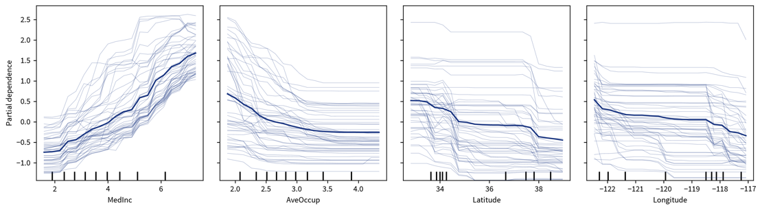
After we’ve identified which features are important for a model in general, we can dig deeper to see how each of these features influences the final prediction. A simple way to accomplish this is with Individual Conditional Expectation (ICE) & Partial Dependence (PD) Plots.

To generate these plots, we take some samples and systematically vary the feature in question for each sample, i.e., set it to many different values within the normal range of values for this feature while keeping everything else about the data points the same. We then observe by how much and in which direction the predictions for these samples change in response to the different values set for the feature.

The ICE plot shows the results for individual samples (thin lines), while the PD plot shows the averaged values (thick line), where the ICE plot can be used to verify that some opposite changes in individual samples are not averaged out in the PD plot:

One big drawback of this approach is that it assumes that the features are independent of each other, i.e., since the features are varied individually, this could otherwise result in unrealistic feature combinations. For example, if one feature is the height of a person (in the range of 60-200cm) and another feature is the weight (30-120kg), then when these features are varied independently, at some point we would evaluate a data point with height: 200cm and weight: 30kg, which seems like a very unhealthy combination.
However, by examining the ICE plot for possibly erratic changes for individual samples, this can usually be spotted. And in general — this goes for all explainability methods — the results should not be over-interpreted, i.e., they are good for showing rough trends, but remember that the plots might also look completely different for a different type of model trained on the same dataset, i.e., be careful before concluding anything about the root causes of a problem based on these results.

Usually, we want a model that reacts smoothly to changes in the input data. Drastic changes in the decision function as a result of minor changes to the input data suggest that a model might be vulnerable to an adversarial attack. Data augmentation can help decrease the model’s sensitivity to noise and other minor variations in the input data.

from sklearn.inspection import partial_dependence

[Local] Model-agnostic: Local Interpretable Model-agnostic Explanations (LIME)

To generate an explanation for a single sample of interest:

Generate a local neighborhood dataset through small perturbations of the sample’s feature vector.
Use the original model to predict labels for these new points, i.e., generate an artificial labeled training set for the local surrogate model.
Train an intrinsically interpretable model (e.g., a linear model) on the neighborhood dataset.
⇒ The decision surface of the original model is very complex, but we assume that it can be approximated locally with a linear function.
Interpret the local surrogate model’s prediction for the sample of interest.

Explaining ML with more ML…

→ lime Python library

Example-Based Explanations

Manually examine some of the data points for which the model predicted a certain target & hopefully notice a pattern…

Prototypes: Representative samples, e.g., cluster centroids.
Optimal inputs: Optimized samples that result in a strong prediction of the given target. For example, in a neural network we can also optimize the input instead of the weights:

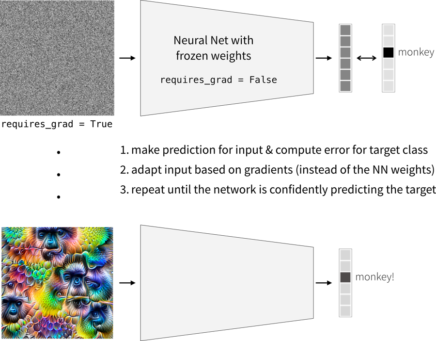Optimal inputs generated with Google’s ‘DeepDream’
Counterfactual examples: Samples with minor modifications that change the prediction. For example, similar to how the optimal inputs are generated, we can also start with an image from a different class (instead of random noise) and adapt it until the network changes its prediction for it.
Adversarial examples: Counterfactual examples where a human doesn’t notice the change.