A Practitioner’s Guide to Machine Learning

Model abuses spurious correlations

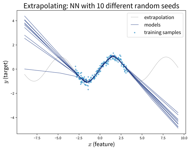
By following the strategies outlined in the previous section, we can find a model that is good at interpolating, i.e., generating reliable predictions for new data points from the same distribution as the training set. However, this does not mean that the model actually picked up on the true causal relationship between the inputs and outputs!

ML models love to cheat & take shortcuts! They will often pick up on spurious correlations instead of learning the true causal relationships. This makes them vulnerable to adversarial attacks and data/domain shifts, which force the model to extrapolate instead of interpolate.

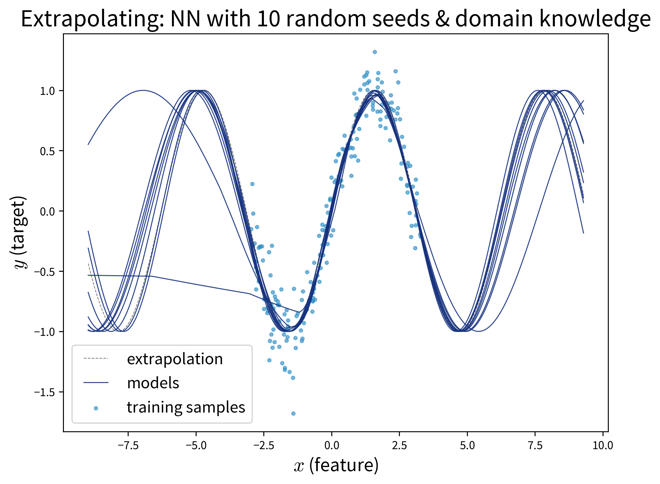
Specifically, models that neither over- nor underfit, i.e., that perfectly capture the relation between inputs and outputs in the given samples, often still fail to extrapolate:

These ten curves were generated by initializing the weights of a FFNN with one hidden layer of 20 units with a ReLU activation with ten different random seeds and then training the network on the data samples. While all these models generalize well on the known data distribution, they can’t produce correct predictions for data points outside of the training domain.

Extrapolation on feature combinations

Please note that only because we might have sampled a large range of values for each individual feature, this does not necessary entail that we’ve also covered all relevant combinations of feature values:

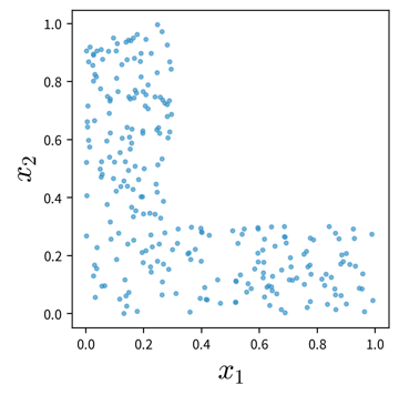
If the two features and their effect on the target are independent of each other (e.g., \(y = ax_1 + bx_2\)), this is not too dramatic, however, if these variables interact in some complicated nonlinear way, this might not be modeled correctly when relevant combinations of feature values weren’t sampled.

When deploying an ML system in production, you also need to replicate the preprocessing steps that were used to clean the training data. For example, if you removed outliers from the initial training set, you need to apply the same rules to sort out anomalies in the production data as well, since otherwise the ML model would be forced to extrapolate on these samples.

When setting up a model, we always have to be clear about whether it is enough that the model is capable of interpolating or whether it might also need to extrapolate every once in a while.

If the model will only be used to generate predictions for new data points from the same distribution as the original training samples and it is unlikely that any data drifts will occur, then a model that has a decent performance on a representative hold-out test set will be sufficient for the task. This might be the case when building a softsensor that just needs to construct a new signal from other fixed inputs in a tightly controlled loop.

However, this assumption seldomly holds in practice and especially in safety-critical situations, such as image recognition in self-driving cars or at security checkpoints, it is vital that the model is robust and can not easily be fooled. Other use cases where it is important that the model picks up on meaningful causal relationships include using a model to identify root causes or generating counterfactual “what-if” forecasts, which also require extrapolation, e.g., when trying to simulate under which conditions a catastrophic event might occur without having observed one in the historical data.

A correct prediction is not always made for the right reasons!

The graphic below is taken from a paper where the authors noticed that a fairly simple ML model (not a neural network) trained on a standard image classification dataset performed poorly for all ten classes in the dataset except one, horses. When they examined the dataset more closely and analyzed why the model predicted a certain class, i.e., which image features were used in the prediction (displayed as the heatmap on the right), they noticed that most of the pictures of horses in the dataset were taken by the same photographer and they all had a characteristic copyright notice in the lower left corner.

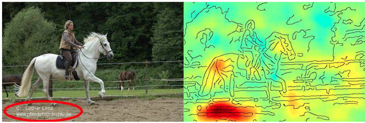
Lapuschkin, Sebastian, et al. “Analyzing classifiers: Fisher vectors and deep neural networks.” IEEE Conference on Computer Vision and Pattern Recognition. 2016.

By relying on this artifact, the model could identify what it perceives as “horses” in this dataset with high accuracy — both in the training and the test set, which includes pictures from the same photographer. However, of course the model failed to learn what actually defines a horse and would not be able to extrapolate and achieve the same accuracy on other horse pictures without this copyright notice. Or, equally problematic, one could add such a copyright notice to a picture of another animal and suddenly the model would mistakenly classify this as a horse, too. This means, it is possible to purposefully trick the model, which is also called an “adversarial attack”.

This is by far not the only example where a model has “cheated” by exploiting spurious correlations in the training set. Another popular example: A dataset with images of dogs and wolves, where all wolves were photographed on snowy backgrounds and the dogs on grass or other non-white backgrounds. Models trained on such a dataset can show a good predictive performance without having learned the true causal relationship between the features and labels.

To catch these kinds of mishaps, it is important to

a) critically examine the test set and hopefully notice any problematic patterns that could result in an overly optimistic performance estimate, and
b) interpret the model and explain its predictions to see if it has focused on the features you (or a subject matter expert) would have expected (as they did in the paper above).

Adversarial Attacks: Fooling ML models on purpose

An adversarial attack on an ML model is performed by asking the model to make a prediction for an input that was modified in such a way that a human is unaware of the change and would still arrive at a correct result, but the ML model changes its prediction to something else.

For example, while an ML model can easily recognize the ‘Stop’ sign from the image on the left, the sign on the right is mistaken as a speed limit sign due to the strategically placed, inconspicuous stickers, which humans would just ignore:

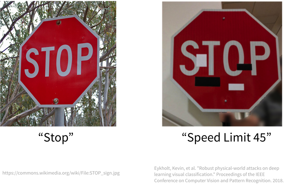
This happened because the model didn’t pick up on the true reasons humans identify a Stop sign as such, e.g., the octagonal form and the four white letters spelling ‘STOP’ on a red background. Instead it relied on less meaningful correlations to distinguish it from other traffic signs.
Convolutional neural networks (CNN), the type of neural net typically used for image classification tasks, rely a lot on local patterns. This is why they are often easily fooled by leaving the global shape of objects, which humans rely on for identification, intact and overlaying the images with specific textures or other high-frequency patterns to trick the model into predicting a different class.

GenAI & Adversarial Prompts

Due to their complexity, it is particularly difficult to control the output of generative AI (GenAI) models such as ChatGPT. While they can be a useful tool in human-in-the-loop scenarios (e.g., to draft an email or write code snippets that are then checked by a human before they see the light of day), it is difficult to put the necessary guardrails in place to ensure the chatbot can’t be abused in the wild.

A Chevrolet car dealer that tried to use ChatGPT in their customer support chat is just one of many examples where early GenAI applications yielded mixed results at best:

Screenshot: https://twitter.com/ChrisJBakke/status/1736533308849443121 (12.1.2024)

Learning causal models

Finding robust causal models that capture the true ‘input → output’ relationship in the data is still an active research area and a lot harder than learning a model that “only” generalizes well to the test set.

Specifically, this requires knowledge of two things:

Which input features should be included in the model, i.e., which variables have a causal impact on the target. In practice, this can be complicated by the fact that we might not be able to measure all of these variables directly and have to rely on proxy values.
What kind of model best captures the true causal relationship, e.g., if the relationship between inputs and target is nonlinear, then a linear model wont be enough. One possibility here is to introduce domain knowledge into the design of a neural network architecture.

Like in the initial example, these ten curves were generated by initializing the weights of a FFNN with one hidden layer of 20 units with a ReLU activation with ten different random seeds and then training the network on the data samples, only this time after the last layer a \(sin()\) activation was applied to the output. By including domain knowledge, we get much closer to the true causal relationship and can extrapolate beyond the training domain (to some extent).

The following example is adapted from: “Elements of Causal Inference” by Jonas Peters, Dominik Janzig, and Bernhard Schölkopf (2017).
See also Jonas Peters' great lecture series on causality. You can also play around with this example yourself in the causal model notebook.

Example: Learning a causal model

Assume this is the true causal graph of some process, where the nodes represent different variables and the edges specify their (linear) influence on one another:

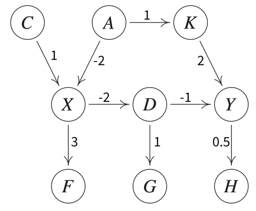
Please note that individual nodes in a causal graph can also represent hidden variables, i.e., process conditions that can not be directly observed, e.g., for which one might want to build a softsensor.

Based on the above stated relationships, we can generate a dataset, where each variable additionally depends on an independent (w.r.t. the other variables) normally distributed noise component. This means for each sample some process conditions are set independently (C and A) while for others the value partially depends on the values already set for the other variables.

n = 20000
C =              1.0 * np.random.randn(n)
A =              0.8 * np.random.randn(n)
K = A          + 0.1 * np.random.randn(n)
X = C - 2 * A  + 0.2 * np.random.randn(n)
F = 3 * X      + 0.8 * np.random.randn(n)
D = -2 * X     + 0.5 * np.random.randn(n)
G = D          + 0.5 * np.random.randn(n)
Y = 2 * K - D  + 0.2 * np.random.randn(n)
H = 0.5 * Y    + 0.1 * np.random.randn(n)

Since the dependencies between the variables are linear, the optimal model type to learn any ‘input → output’ relation on this dataset is a linear regression model. The true coefficients that this model should find for one input variable are the values on the edges on the way from this variable’s node to the target node multiplied with each other, e.g., for X (input) on Y (target) this would be -2 (from X to D) times -1 (from D to Y), i.e., 2.

Depending on which variables we include as input features, the models is or isn’t able to learn the correct coefficients:

# (1) missing relevant input feature K -> wrong coefficient for X
R^2 (train): 0.844; (test): 0.848 => Y ~  0.001 + 1.285 * X
# (2) all the right input features -> correct coefficients
R^2 (train): 0.958; (test): 0.959 => Y ~  0.003 + 2.003 * X + 2.010 * K
# (3) additional input feature D, which has a more direct influence on Y than X
R^2 (train): 0.994; (test): 0.994 => Y ~ -0.002 - 0.015 * X + 1.998 * K - 1.007 * D
# (4) additional input feature H, which is dependent on (i.e., highly correlated with) Y
R^2 (train): 0.995; (test): 0.995 => Y ~  0.001 + 0.242 * X + 0.245 * K + 1.759 * H
# (5) additional input feature G that is not directly causal of Y, but dependent on D
R^2 (train): 0.977; (test): 0.976 => Y ~  0.004 + 0.978 * X + 2.002 * K - 0.510 * G

Often the best predictive model is not the true causal model (e.g., (4)) and especially regularized models, which try to explain the target with as few variables as possible, often choose variables dependent on the target (such as H) as the single best predictor instead of relying on multiple true causal influences (e.g., notice how K and X already have much lower coefficients in (4)).
But only the causal models are robust to data drifts and can extrapolate:

# Changed equations to generate test data (notice larger noise component)
X = C - 2 * A  + 2.0 * np.random.randn(n)
H = 0.5 * Y    + 1.0 * np.random.randn(n)

# model (2): true relationship between X and Y -> test performance equally good
R^2 (train): 0.958; (test): 0.987 => Y ~ 0.003 + 2.003 * X + 2.010 * K
# model (4): variable dependent on but not causal of Y -> test performance a lot worse
R^2 (train): 0.995; (test): 0.866 => Y ~ 0.001 + 0.242 * X + 0.245 * K + 1.759 * H

But unfortunately none of the models can handle a concept drift, i.e., when the underlying process, from which the data is sampled, changes:

# Changed equation to generate test data (notice the reversed sign for X on the way to Y)
D =  2 * X     + 0.5 * np.random.randn(n)

# model (2): causal relationship between X and Y changed -> test performance catastrophic
R^2 (train): 0.958; (test): -1.797 => Y ~ 0.003 + 2.003 * X + 2.010 * K

In this case only retraining the model on new data helps to recover the performance.

⇒ If the goal is to find a good predictive model, use as input variables the Markov blanket of the target variable, i.e., its parent nodes, child nodes, and the other parent nodes of these child nodes (in the above example, to predict Y this would be D and K (parent nodes) and H (child node that has no other parents)).
⇒ If the goal is to find a causal model that can extrapolate, use as input variables only the parent nodes of the target variable.

Residual Plots

Residual plots can give us a hint as to whether or not we might be missing important input variables in the model.

In regression problems we assume that the input variables explain all important external influences on the target and what remains is just random noise. I.e., as we predict the target as:

\[\hat{y} = b + w_1x_1 + w_2x_2 + ... + w_dx_d\]

we assume that the true process that generated \(y\) looked like this:

\[y = b + w_1x_1 + w_2x_2 + ... + w_dx_d + \epsilon\]

where \(\epsilon \in \mathcal{N}(0, \sigma)\) is the unexplained random noise with mean 0 and standard deviation \(\sigma\), which is assumed to be independent of all other factors.

By plotting the residuals (i.e., prediction errors) \(y_i - \hat{y}_i\) against the predicted targets \(\hat{y}_i\) and other variables and observing whether or not these residuals show distinctive patterns or really look like random noise, we can check whether the model is missing important additional input variables.

For example, from the example above for model (1), i.e., when using only X as an input to predict Y, the residuals plots looks like this:

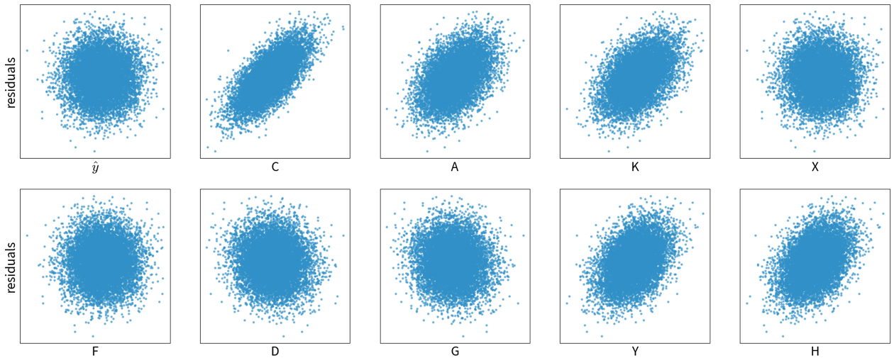
The residuals here are correlated with several other variables, which means we should probably include one of them as an additional input feature.

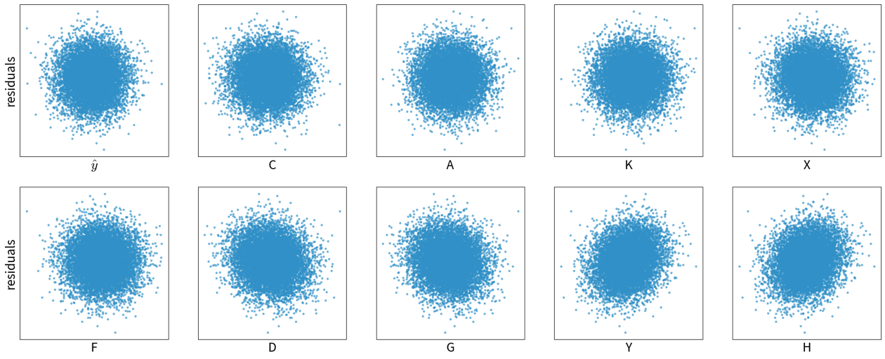
The residuals plots for model (2), i.e., when using both X and K as features, on the other hand, show randomly distributed residuals, which means, we’re at least not missing some obvious influencing factors:

When working with time series data, you should also check for autocorrelation between the residuals, i.e., it should not be possible to use the residual at time point t to predict the next residual at t+1.