Reinforcement Learning
Finally, we come to the last main category of ML algorithms besides unsupervised and supervised learning: reinforcement learning.
- Main idea
-
Agent performs actions in some environment and learns their (state-specific) consequences by receiving rewards.
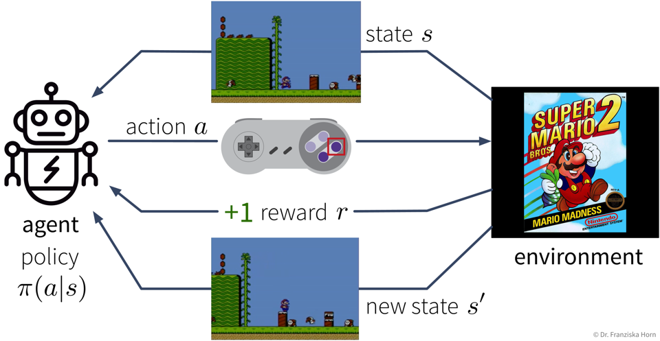
Goal: Maximize the cumulative reward (also called return), i.e., the sum of the immediate rewards received from the environment over all time steps in an episode (e.g., one level in a video game).
The difficult thing here is that sometimes an action might not result in a big immediate reward, but is still crucial for the agent’s long-term success (e.g., finding a key at the beginning of a level and the door for which we need the key comes much later). This means the agent needs to learn to perform an optimal sequence of actions from delayed labels.
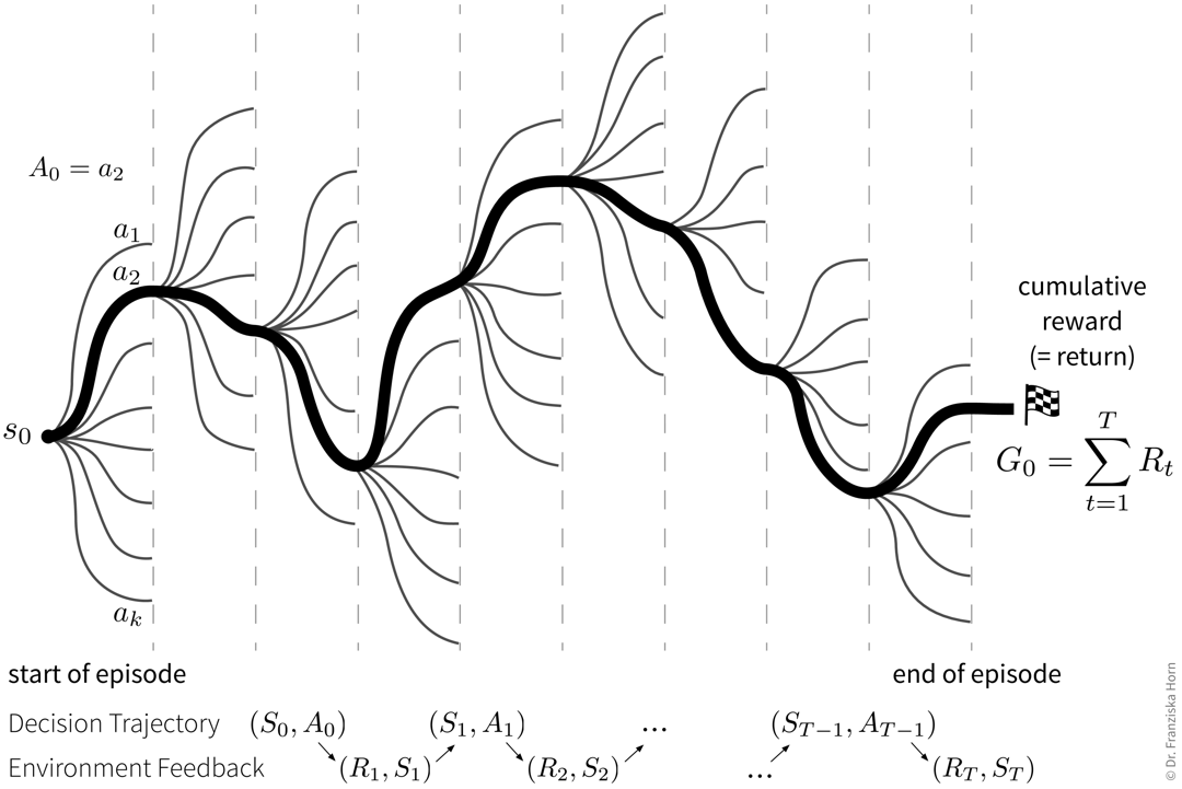
The agent’s decision trajectory basically defines one path among a bunch of different possible parallel universes, which is then judged in the end by the collected return:
- Immediate rewards vs. long-term value of states
-
To make decisions that are good in the long run, we’re more interested in what being in a state means w.r.t. reaching the final goal instead of receiving immediate rewards:
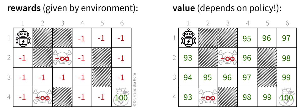 Left: This is a simple "grid world", where an agent can move up, down, left, or right through the states. This small environment contains three terminal states (i.e., when the agent reaches one of them, the episode ends): Two states mean "game over" with an infinite negative reward, while reaching the state in the lower right corner means receiving a large positive immediate reward. When the agent resides in any of the other (reachable) states, it receives a small negative reward, which is meant to "motivate" the agent to go to the goal state as quickly as possible. However, knowing only the immediate reward for each state is not very helpful to decide which action to take next, since in most states, the reward for moving to any of the surrounding states or staying in place would be the same. Therefore, what the agent needs to learn in order to be able to choose an action in each state that has the potential of bringing it closer to the goal state, is the value of being in each state. Right: The value of a state is the expected return when starting from this state. Of course, the expected return is highly dependent on the agent’s policy \(\pi\) (i.e., the actions it takes), e.g., if the agent would always move to the left, then it would never be able to reach the goal, i.e., the expected return starting from any state (except the goal state itself) would always be negative. If we assume an optimal policy (i.e., the agent always takes the quickest way to the goal), then the value of each state corresponds to the ones shown in the graphic, i.e., for each state "100 minus the number of steps to reach the goal from here". Knowing these values, the agent can now very easily select the best next action in each state, by simply choosing the action that brings it to the next reachable state with the highest value.
The value of a state \(s\) corresponds to the expected return \(G_t\) when starting from state \(s\):
The most naive way to calculate \(V^\pi(s)\) would be to let the agent start from this state several times (depending on how complex the environment is usually several thousand times), observe how each of the episodes play out, and then compute the average return that the agent had received in all these runs starting from state \(s\).
Similarly, we can calculate the expected return when executing action \(a\) in state \(s\):
I.e., here again we could let the agent start from the state \(s\) many times, but this time the first action it takes in this state is always \(a\).
- Exploration/Exploitation trade-off
-
Of course, it would be very inefficient to always just randomly try out actions in any given state and thereby risk a lot of predictable “game over”. Instead, we want to balance exploration and exploitation to keep updating our knowledge about the environment, but at the same time also maximize the rewards collected along the way. This is again inspired by human behavior:
-
→ Exploration: Learn something about the environment (e.g., try a new restaurant).
-
→ Exploitation: Use the collected knowledge to maximize your reward (e.g., eat somewhere you know you like the food).
A very simple strategy to accomplish this is the Epsilon-Greedy Policy:
initialize eps = 1 for step in range(max_steps): if random(0, 1) > eps: pick best action (= exploitation) else: pick random action (= exploration) reduce eps -
- Tabular RL: Q-Learning
-
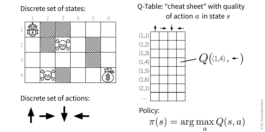
This brings us to the simplest form of RL, tabular RL, where an agent has a finite set of actions to choose from and operates in an environment with a finite set of states (like the grid world from above). Here, we could simply compute the Q-value for each (state, action)-combination as described above, and save these values in a big table. This so-called Q-table then acts as a cheat sheet, since for each state the agent is in, it can just look up the Q-values for all of the available actions and then choose the action with the highest Q-value (when in exploitation-mode):
- Function Approximation: Deep Q-Learning
-
Unfortunately, almost no practical RL application operates in an environment consisting of a finite set of discrete states (and sometimes even the agent’s actions are not discrete, e.g., the steering wheel positions in a self-driving car — but this goes too far here). In video games, for example, each frame is a new state and depending on the complexity of the game, no two frames might be exactly alike. This is where Deep Q-Learning comes in:
Given a state \(s\) (represented by a feature vector \(\mathbf{x}_s\)), predict the Q-value of each action \(a_1 ... a_k\) with a neural network:
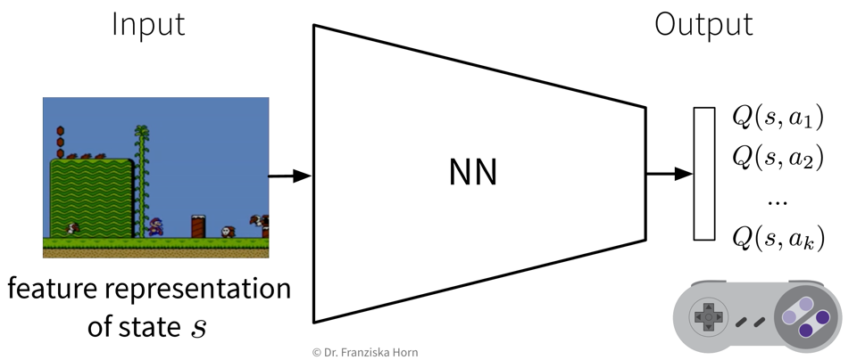
This can be seen as a direct extension of the tabular Q-learning: If we represented our states as one-hot encoded vectors and used a linear network with a single weight matrix that consisted of the Q-table we had constructed before, by multiplying the one-hot encoded vector with the Q-table, the network would “predict” the row containing the Q-values for all actions in this state.
By using a more complex network together with meaningful feature representations for the states, deep Q-learning enables the agent to generalize to unseen states. However, just like in time series forecasting tasks, here again the feature representation of a state needs to include all the relevant information about the past, e.g., in video games (think: old pong game) the feature vector could contain the last four frames to additionally capture the direction of movement.
RL further reading + videos
General theory:
-
Chapters 11+12 from the book Patterns, Predictions, and Actions
-
Lectures by David Silver (from DeepMind)
-
Stanford RL course (with video lectures)
-
Book about RL (with lots of math)
Words of caution (recommended for everyone):
RL in action:
-
Robot arm data collection (by Google)
-
Playing video games with Layer-wise Relevance Propagation (LRP) to show the evolution of strategy