A Practitioner’s Guide to Machine Learning

Time Series Forecasting

In the chapter on data, where we discussed what can be considered ‘one data point’, you’ve already encountered some tasks that involve time series data. Now we’re looking into possibly the most difficult question that one can try to solve with time series data, namely predicting the future.

In time series forecasting, sometimes also called “predictive analytics”, the goal is to predict the future time course of a variable (i.e., its values for \(t' > t\)) from its past values (and possibly some additional information). This is, for example, used in Predictive Maintenance, where the remaining life span or degradation of important process components is forecast based on their past usage and possibly some future process conditions:

One predictive maintenance problem coming up over and over again in the chemical production industry is trying to predict the remaining activity or lifetime of a catalyst (a critical component in a chemical plant that facilitates the reaction; visualized as the purple line) under different process conditions (which are planned for the future; blue and green lines). For example, the catalyst might decay faster, if the process is run at a higher temperature. If the weekend is coming up, a predictive maintenance model could be used to estimate the temperature at which the process should be run such that the catalyst lasts until the next Monday, when the crew to replace it is back.

Predictive Maintenance Example Paper:
Bogojeski, M., et al. “Forecasting industrial aging processes with machine learning methods.” Computers and Chemical Engineering 144 (2021): 107123. (arXiv:2002.01768)

Input and Target Variables

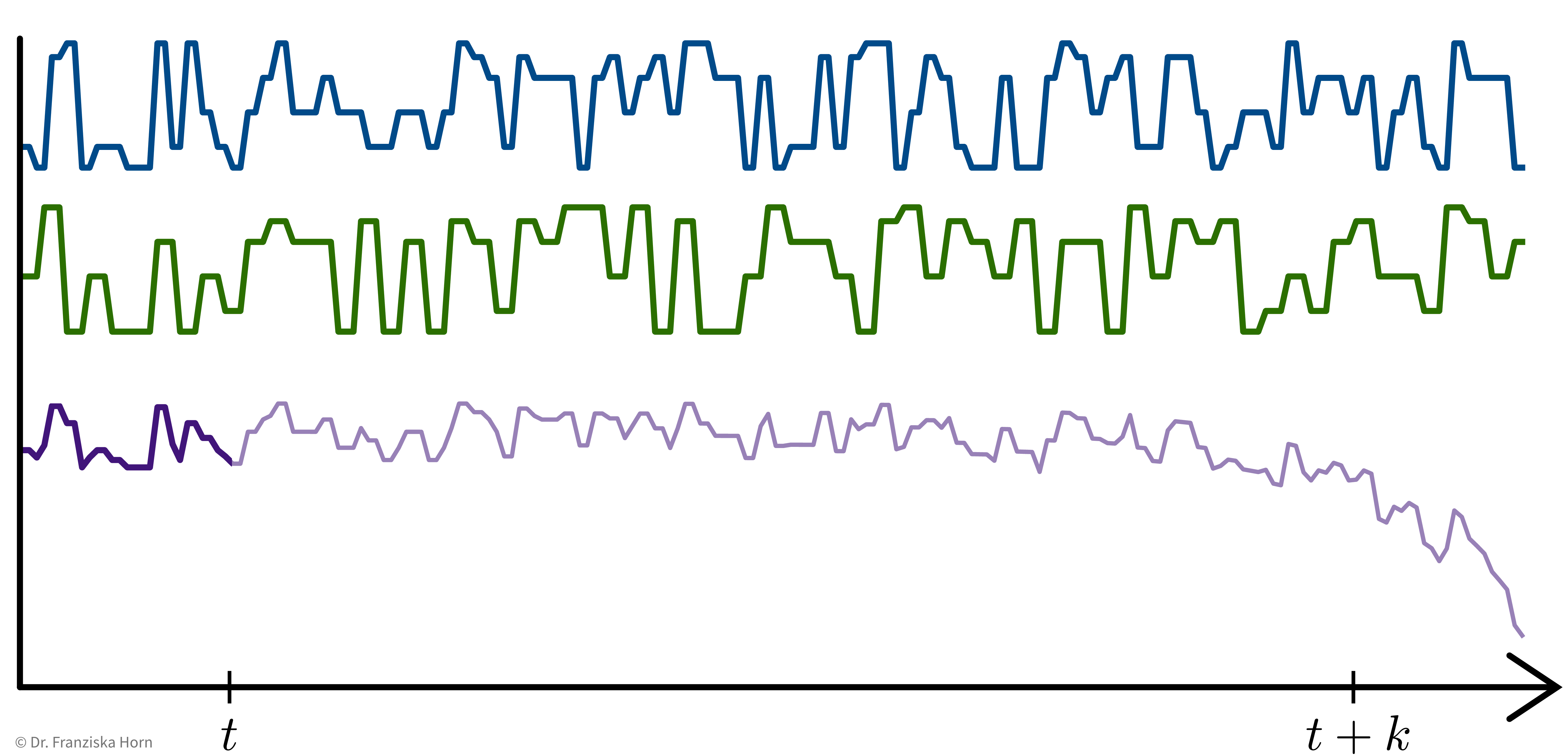
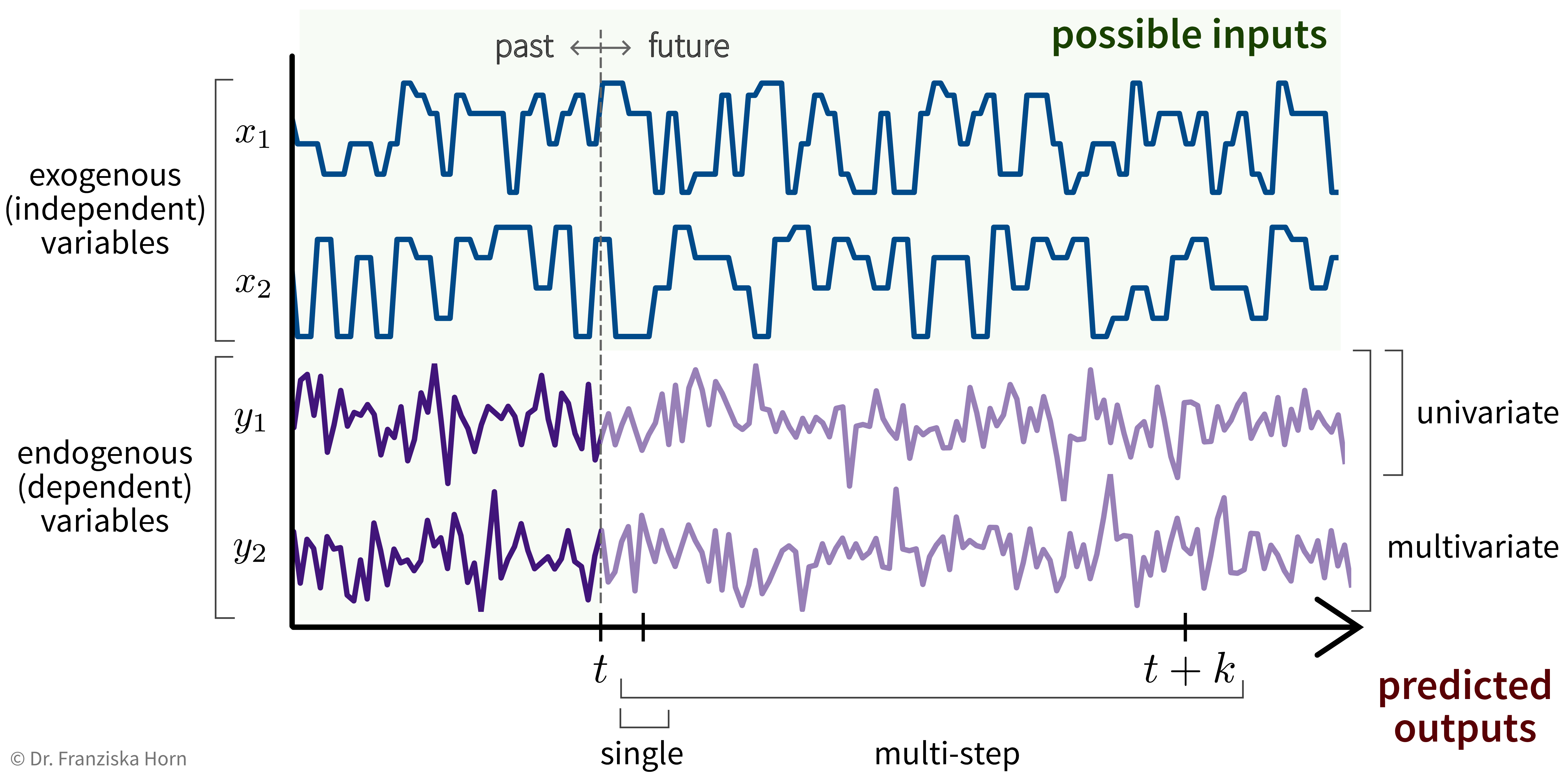
Basically, we can think of time series forecasting as a supervised learning problem with more complicated inputs & outputs:

Depending on the task (i.e., what we want to forecast), we either have a univariate forecasting problem (if we only need to predict the development of a single variable) or a multivariate problem (i.e., with multiple target variables). Additionally, it is important to note for how many time steps into the future the variables need to be forecast: In the easiest case, only the next time step needs to be predicted, but it might also be necessary to predict a fixed window of \(k\) time steps into the future, and sometimes the prediction horizons might even be of varying lengths. In any case, we should always try to make use of as much (relevant) information as possible when making forecasts. In principle, all values from the past can be used as input features, especially those from the target variable(s) (→ see also auto-regressive models, e.g., ARIMA). What is often overlooked, however, is all the additional information about the future that can be used as inputs as well, provided that these values are independent of the targets, i.e., exogenous variables outside of the system.

For example, let’s say we own a small cafe and want to predict how much ice cream we are likely to sell tomorrow. Certainly, the amount of ice cream we’ve sold yesterday or on the same day last week will be useful input features, but additionally, for example, the weather forecast for tomorrow or whether or not there is a holiday or some special event happening would be useful predictive information that should not be ignored and that can be used since these are independent variables.

Know your data: Beware of hidden feedback loops!

In this predictive maintenance example, the pressure in some pipes indicates how much residual material has built up on the walls of the pipes (→ fouling) and the task is to predict when these pipes need to be cleaned again, i.e., when the next maintenance event is due.

What are input features, what are targets?: While in general many future process conditions (e.g., the planned amount of product that should be produced in the next weeks), can be used as input variables at \(t' > t\), this does not hold for the process condition ‘temperature’ in this example, since it is not a true exogenous variable, even though it could theoretically be set independently. In the historical data, the value of the temperature at \(t+1\) is dependent on the target variable (pressure) at \(t\), therefore, if we want to forecast the target for more than one time step, only the past values of temperature can be used as input features.

We need a feature vector for every time point we want to make a prediction about. Think about what it is we’re trying to predict and what values could influence this target variable, i.e., what inputs are needed such that we have all the required information to make the prediction. Especially when using stateless models (see below), the feature vectors need to capture all the relevant information about the past.

Possible Input Features

Known information about future (e.g., weather forecast, planned process conditions).
Auto-regressive: Lagged (target) variable (i.e. values at \(t' \leq t\)).
❗️ Don’t use the predicted target value for this (in a multi-step forecast) – errors accumulate!
Account for cyclical (e.g., seasonal) trends → check auto-correlation or spectral analysis.
For example, a cafe might sell more ice cream during the summer or it could be located next to a school and therefore sell more on days the kids come by in their lunch break:

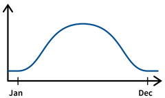
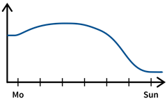
→ Include categorical variables month and day_of_week.
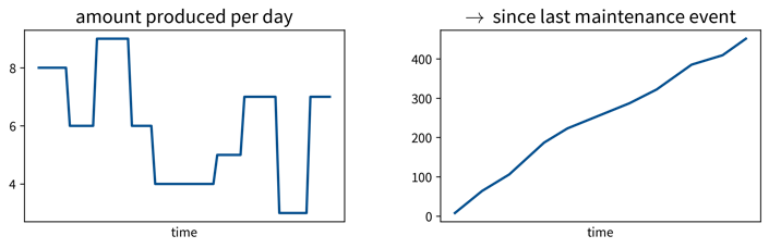
For predictive maintenance: hours / integral of input variable since last maintenance event (maybe take log).

→ For more ideas: tsfresh library, time series analysis blog posts

Stateless vs. Stateful Models

When dealing with time series data, one should always think carefully about how complex the dependencies between the past and future process values in the respective forecasting task are.
For example, when trying to predict spontaneous events, like a sudden increase in the emissions produced in the process, then the relevant time window into the past, when the process conditions might have had an influence on this target variable, would be very short, i.e., only the process values from time \(t\) need to be included in the input feature vector to predict the anomalous event at time \(t+1\).
For other prediction tasks, what happened over a longer (but uniquely determined) interval might be relevant, but can be summarized with simple features. For example, in a production process, one might want to predict the quality of the final product that is produced within a fixed time interval. In this case, the process conditions during the time interval where the respective product is produced will be important for the prediction, but the process conditions during the time where the previous product was produced are most likely not relevant. Additionally, it would be enough to compute only some summary statistics (like mean/max/min values of the process conditions during the time interval of interest) and use these as input features to capture all the relevant information.
The third case are prediction tasks for which it is necessary to consider very long time windows, often of varying lengths, with some complex long-ranging dependencies between the process conditions at different time points. For example, in some predictive maintenance tasks, the decay of the critical process component might not happen in some linear fashion (unlike, for example, a light bulb, which might have some fixed life expectancy and one only needs to count the number of hours it was turned on up to now to estimate when it needs to be replaced). Instead, there exist more complex dependencies, for example, the component might decay faster if it is already in a poor state. Therefore, if some unfortunate combination of process conditions lead to a strain on the component early on, it might have to be replaced a lot sooner than under otherwise identical conditions without this initial mishap, i.e., the order of events matters a lot, too.

Depending on how complex the dependencies are between the process values over time, it will be more or less complicated to construct feature vectors that capture all the relevant information to make accurate predictions. In general, one should always try to come up with features that contain all the relevant information about the past, i.e., that fulfill the Markov assumption that given this information the future is otherwise independent of the history of the process: For example, if we knew the number of hours a light bulb was turned on up to now, we would have a complete picture about the state the light bulb is currently in; everything else that happened in the past, like how many people were in the room while the light was on, is irrelevant for the state of the light bulb. Another example is the current position of pieces on a chess board: To plan our next move, we don’t need to know the exact order in which the pieces were moved before, but only the position of all the pieces right now.

If we are able to derive such input features, we can use a stateless model for the prediction (e.g., any of the supervised learning models we’ve discussed so far except RNNs), i.e., treat all data points as independent regardless of where in time they occurred. If it is not possible to construct such an informative feature vector that captures all the relevant information about the past, e.g., because of complex long-ranging dependencies that can not be adequately captured by simple summary statistics, then we have to use a stateful model (e.g., a form of Recurrent Neural Network (RNN)), which internally constructs a full memory of the history of the process, i.e., it keeps track of the current state of the process.

Whether to use a stateless or stateful model is also an important consideration when dealing with other kinds of sequential data such as text. Analogous to the three scenarios described above, we can also find similar cases for natural language processing (NLP) problems that either benefit from the use of stateful models or where a simple stateless model is enough:

Spontaneous event: Trigger word detection for smart speakers: A simple classification task for which only the last 1-2 spoken words, i.e., the audio signal from a time window of a few seconds, are relevant.
Fixed interval & summary features: Text classification, e.g., determining the category of a newspaper article (e.g., ‘sports’ or ‘politics’): While here a longer span of text needs to be considered to make the prediction, a simple TF-IDF vector is usually sufficient to represent the contents of the whole document, since such categories can easily be identified by simply checking whether the terms “soccer” or “politician” occur more often in the current article. Furthermore, the span of text that is relevant for the task is fixed: we only need to consider the current article and it can be considered independent of the articles written before it.
Complex long-ranging dependencies: For some tasks like sentiment analysis or machine translation, it doesn’t just matter which words occurred in a text, but also in which order and what their larger surrounding context was.

→ While for 1. and 2. a stateless model will do just fine, for 3. the best performance is achieved with a stateful model that can keep track of the more complex dependencies.

TL;DR: Which type of model should we use?

How much does the future depend on the past?
a) Values at \(t\) or simple summary statistics are sufficient as input features to predict \(t' > t\).
b) There exist complex long-ranging dependencies between past and future values and the order of events matters.
How many time steps into the future do we need to predict?
a) A fixed, small window of \(1\) or \(k\) steps.
b) Arbitrarily long prediction horizons.

If only a):
→ Stateless model, e.g., linear model, FFNN, random forest, …
If any b):
→ Stateful model, e.g., recurrent neural network (RNN)

When working with time series data, the train, validation, and test data splits should always be in chronological order, i.e., the model is trained on the oldest time points and evaluated on more recent samples to get a realistic performance estimate, especially in cases where the data changes over time, e.g., due to smaller changes in the underlying process.

Output prediction with stateless models (e.g., linear regression, FFNN)

Only predict for a fixed time window of 1 or k steps:

Univariate, single-step prediction:

\[[\underbrace{\quad y_1 \quad}_{t' \,\leq\, t} | \underbrace{\, x_1 \, | \, x_2 \, }_{t+1} ] \; \to \; [\underbrace{y_1}_{t+1}]\]
Multivariate, single-step prediction:

\[[\underbrace{\quad y_1 \quad | \quad y_2 \quad}_{t' \,\leq\, t} | \underbrace{\, x_1 \, | \, x_2 \, }_{t+1} ] \; \to \; [\underbrace{\, y_1 \, | \, y_2 \, }_{t+1}]\]
Multivariate, multi-step prediction:

\[[\underbrace{\quad y_1 \quad | \quad y_2 \quad}_{t' \,\leq\, t} | \underbrace{\quad\quad x_1 \quad\quad | \quad\quad x_2 \quad\quad }_{t+1\, ...\, t+k} ] \; \to \; [\underbrace{\quad\quad y_1 \quad\quad | \quad\quad y_2 \quad\quad }_{t+1\, ...\, t+k}]\]

Output prediction with stateful models (e.g., RNN, LSTM, GRU, Echo State Network): The model builds up a memory of the past by mirroring the actual process, i.e., even if we don’t need the prediction at some time step \(t-5\), we still need to feed the model the inputs from this time step so that it can build up the appropriate hidden state.

Multivariate, multi-step prediction:

\[\begin{aligned} ...\\ t-1:\quad [\, x_1 \, | \, x_2 \,]\; &\to \; [\, y_1 \, | \, y_2 \,]\\ \text{memory state buildup} \quad\quad\quad\quad t:\quad [\, x_1 \, | \, x_2 \,]\; &\to \; [\, y_1 \, | \, y_2 \,]\\ ---------------------&------\\ \text{prediction} \quad\quad\quad\quad\quad t+1:\quad [\, x_1 \, | \, x_2 \,]\; &\to \; [\, y_1 \, | \, y_2 \,]\\ t+2:\quad [\, x_1 \, | \, x_2 \,]\; &\to \; [\, y_1 \, | \, y_2 \,]\\ ...\\ t+k:\quad [\, x_1 \, | \, x_2 \,]\; &\to \; [\, y_1 \, | \, y_2 \,] \end{aligned}\]