A Practitioner’s Guide to Machine Learning

Outlier / Anomaly Detection

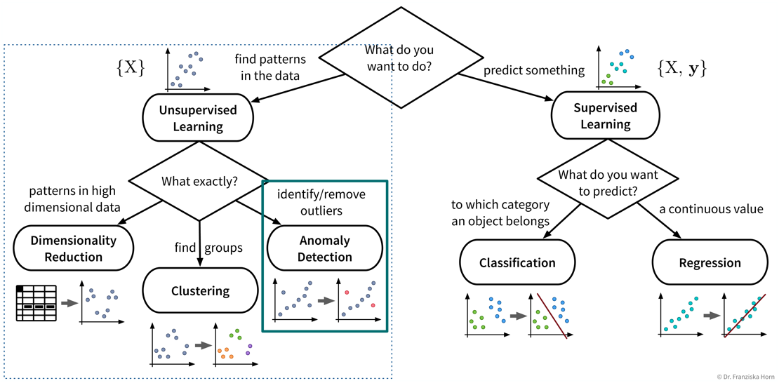
Next up on our list of ML tools is anomaly or outlier detection:

Useful for

Detecting anomalies for monitoring purposes, e.g., machine failures or fraudulent credit card transactions.
Removing outliers from the dataset to improve the performance of other algorithms.

Things to consider when trying to remove outliers or detect anomalies:

Does the dataset consist of independent data points or time series data with dependencies?
Are you trying to detect
- outliers in individual dimensions? For example, in time series data we might not see a failure in all sensors simultaneously, but only one sensor acts up spontaneously, i.e., shows a value very different from the previous time point, which would be enough to rule this time point an anomaly irrespective of the values of the other sensors.
- multidimensional outlier patterns? Individual feature values of independent data points might not seem anomalous by themselves, only when considered in combination with the data point’s other feature values. For example, a 35 \(m^2\) apartment could be a nice studio, but if this apartment supposedly has 5 bedrooms, then something is off.
Are you expecting a few individual outliers or clusters of outliers? The latter is especially common in time series data, where, e.g., a machine might experience an issue for several minutes or even hours before the signals look normal again. Clusters of outliers are more tricky to detect, especially if the data also contains other ‘legitimate’ clusters of normal points. Subject matter expertise is key here!
Do you have any labels available? While we might not know what the different kinds of (future) anomalies look like, maybe we do know what normal data points look like, which is important information that we can use to check how far new points deviate from these normal points, also called novelty detection.

Know your data — are missing values marked as NaNs (“Not a Number”) or set to some ‘unreasonable’ high or low value?

Removing outlier samples from a dataset is often a necessary cleaning step, e.g., to obtain better prediction models. However, we should always be able to explain why we removed these points, as they could also be interesting edge cases.
Try to remove as many outliers as possible with manually crafted rules (e.g., “when this sensor is 0, the machine is off and the points can be disregarded”), especially when the dataset contains clusters of outliers, which are harder to detect with data-driven methods.

Please note that some of the data points a prediction model encounters in production might be outliers as well. Therefore, new data needs to be screened for outliers as well, as otherwise these points would force the model to extrapolate beyond the training domain.

Different methods for outlier/anomaly detection

There is no one-size-fits-all solution, but depending on the characteristics of the dataset you might want to experiment with some of these approaches:

Detect outliers in individual feature dimensions:
- Compute the interquartile range (IQR), i.e., the difference between the 75th and 25th percentiles of the data, as \(\text{IQR} = Q_3 - Q_1\), where \(Q_1\) and \(Q_3\) are the lower and upper quartiles. All data points with values outside of the range \([Q_1-1.5\cdot \text{IQR},\; Q_3+1.5\cdot \text{IQR}\)] are considered outliers.
Detect multidimensional outlier patterns, especially in datasets with independent data points (see also sklearn user guide):
- \(\gamma\)-index (see below)
- Local Outlier Factor (from sklearn; similar to the \(\gamma\)-index)
- Isolation Forest (from sklearn; read about decision trees and random forests first)
- One-class SVM (from sklearn; read about kernel methods and normal SVMs first)
- DBSCAN (a clustering algorithm that allows for noise, which would be considered outliers)
Compare actual data points to denoised samples or predicted values:
- Use (kernel) PCA or an auto-encoder neural network architecture to first compress a sample and then reconstruct it in order to remove noise. If the denoised data point deviates a lot from the original sample, it is probably an anomaly.
- For time series data: model the expected course of an individual time series, e.g., using a moving window average or an ARIMA model (see section on time series forecasting for more details), and then compare how much a time point deviates from this predicted value.
Get creative: you know your data best — define rules and custom anomaly KPIs based on your domain knowledge, e.g., set thresholds for what would be considered unrealistic feature values etc.

\(\gamma\)-index

Harmeling, Stefan, et al. “From outliers to prototypes: ordering data.” Neurocomputing 69.13-15 (2006): 1608-1618.

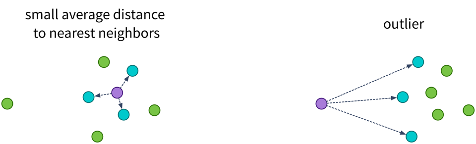
Main idea: Compute the average distance of a point to its k nearest neighbors:
→ Points with a large average distance are more likely to be outliers.
⇒ Set a threshold for the average distance when a point is considered an outlier.

This toy example in 2D, but of course the Euclidean distance between the points can also be computed in higher dimensional features spaces.

import numpy as np
from sklearn.metrics import pairwise_distances

def gammaidx(X, k):
    """
    Inputs:
        - X [np.array]: n samples x d features input matrix
        - k [int]: number of nearest neighbors to consider
    Returns:
        - gamma_index [np.array]: vector of length n with gamma index for each sample
    """
    # compute n x n Euclidean distance matrix
    D = pairwise_distances(X, metric='euclidean')
    # sort the entries of each row, such that the 1st column is 0 (distance of point to itself),
    # the following columns are distances to the closest nearest neighbors (i.e., smallest values first)
    Ds = np.sort(D, axis=1)
    # compute mean distance to the k nearest neighbors of every point
    gamma_index = np.mean(Ds[:, 1:(k+1)], axis=1)
    return gamma_index

# or more efficiantly with the NearestNeighbors class
from sklearn.neighbors import NearestNeighbors

def gammaidx_fast(X, k):
    """
    Inputs:
        - X [np.array]: n samples x d features input matrix
        - k [int]: number of nearest neighbors to consider
    Returns:
        - gamma_index [np.array]: vector of length n with gamma index for each sample
    """
    # initialize and fit nearest neighbors search
    nn = NearestNeighbors(n_neighbors=k).fit(X)
    # compute mean distance to the k nearest neighbors of every point (ignoring the point itself)
    # (nn.kneighbors returns a tuple of distances and indices of nearest neighbors)
    gamma_index = np.mean(nn.kneighbors()[0], axis=1)  # for new points: nn.kneighbors(X_test)
    return gamma_index

Pros

Conceptually very simple and easy to interpret.

Careful

Computationally expensive for large datasets (distance matrix: \(\mathcal{O}(n^2)\)) → compute distances to a random subsample of the dataset or to a smaller set of known non-anomalous points instead.
Normalize heterogeneous datasets before computing distances!
Know your data: does the dataset contain larger clusters of outliers? → k needs to be large enough such that a tight cluster of outliers is not mistaken as prototypical data points.

Extension for time series data: don’t identify the k nearest neighbors of a sample based on the distance of the data points in the feature space, but take the neighboring time points instead.

You’ve found an outlier — now what?